Final Project: Design of an Electric Vehicle

Create a MATLAB model of electric car which uses a battery and a DC motor. Choose suitable blocks from Powertrain block set. Prepare a report about your model including following:

Objectives:

1. System level configurations

2. Model parameters

3. Results

4. Conclusion

Aim:

To create a MATLAB model of electric car which uses a battery,DC motor and suitable blocks from powertrain blockset.

Objectives:

• To make a most simple and low run time vehicle model using individual components models
• To check out performance parameters like Speed,SOC,Current etc with various drive cycles
• To play with: Motor Power,Vehicle body (Rolling resistance ,air drag,Weight),inputs

Drivetrain & Powertrain:

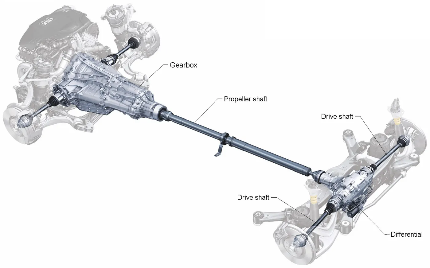
• The main difference between a drive train and powertrain is that the powertrain generates the power using engine or motor and the drivetrain distributes that power to the car.
• A group of drivetrain parts is connected to the engine to move the wheels and other moving parts
• A drivetrain commonly consist of transmission, differential, driveshaft, axles, CV joints, and wheels.

Order of how power is generated and delivered by the drivetrain:

• The engine will create power to power a flywheel
• That flywheel works with the transmission to manage the amount of power distributed to various other parts of the drivetrain
• The driveshaft rotates to produce power to a differential
• After that the differential delivers power from all those driveshaft parts the car moves

• In the powertrain,Engine has many moving parts and it is connected with the drivetrain.
• Powertrain converts the kinetic energy in to propulsion movement
• If one of the parts fails the car experience uncommon rattling and shaking.

Main parts of EV:

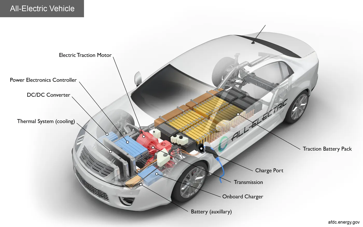
• Traction battery pack:

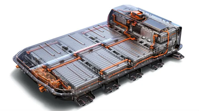
In a pure ev or Battery Electric Vehicle (BEV) the main source of energy is from a battery pack.

Non–plug-in hybrid cars can have battery capacities between 0.65 kWh (2012 Honda Civic Hybrid) and 1.8 kWh (2001 Toyota Prius).
Plug-in hybrid cars can have battery capacities between 4.4 kWh (2012 Toyota Prius Plug-in Hybrid) and 34 kWh (Polestar 1).
All-electric cars can have battery capacities between 6.0 kWh (2012 Renault Twizy) and 100 kWh (2012 Tesla Model S and 2015 Tesla Model X).

Batteries used in evs:

1. Lead acid battery
2. Lithium ion battery
3. Lithium polymer battery
4. Nickel Cadmium battery
5. Nickel metal hydride
6. Solid state batteries
7. Graphene batteries etc

The other sources of power are high speed flywheels and ultra capacitors.

• Auxilary battery:

In EVs auxilary battery provides power to the low power devices,accesories and other auxilary devices

• Traction motor:

Converts electrical energy in to mechanical rotational energy.Used to give tractive power to wheels

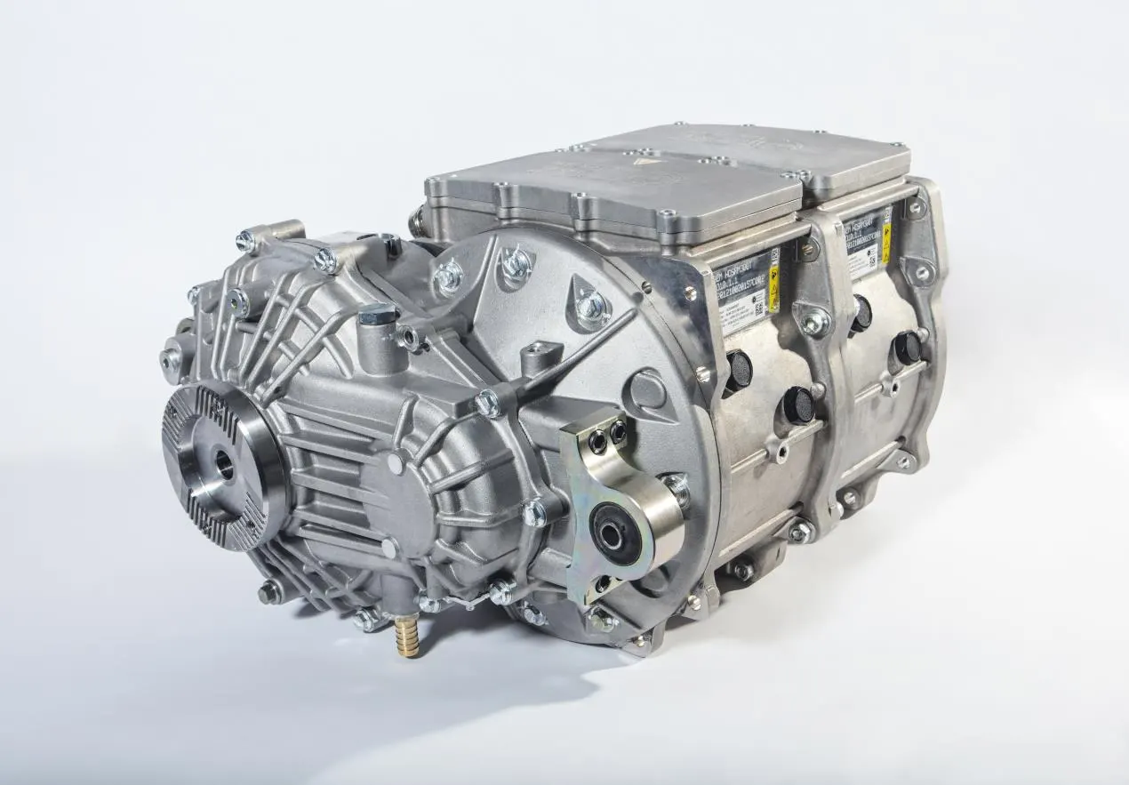
Motors used in EVs:

1. Brushed DC motors
2. Brushless DC motors(BLDC)
3. Permanent Magnet Synchronous Motor(PMSM)
4. Induction motors
5. Switched Reluctance Motors(SRM)
6. Synchronous Reluctance Motor(SyRM)
7. Axial Flux Interior Permanent Motor(AFIPM)

• Power converters
• Power electronics controller
• Onboard charger
• Thermal cooling system

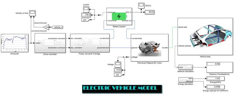
Block Diagram:

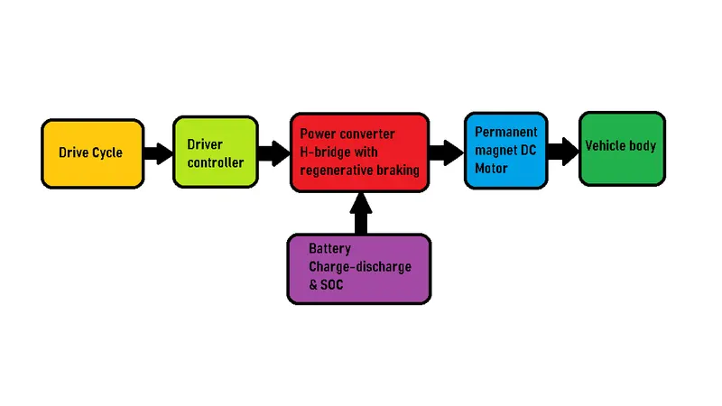
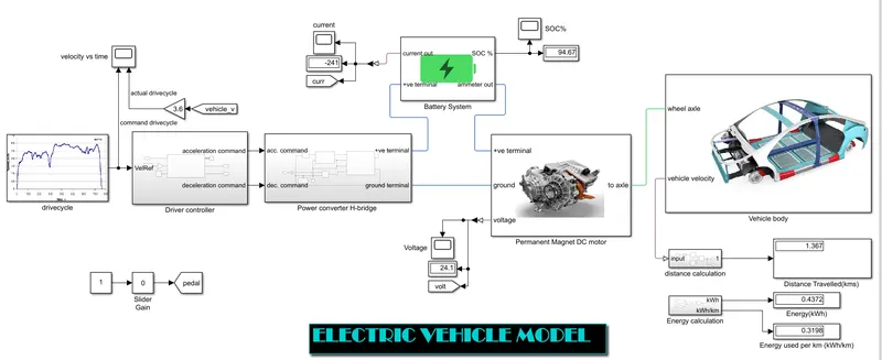
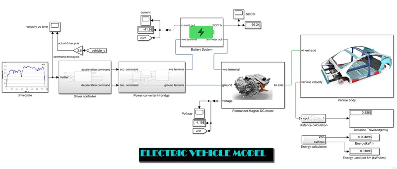
• In this matlab ev modelling ,it contains a drive cycle block where we provide a specific drive cycle which is a graph plotted between Velocity in y-axis and time in x-axis.
• Then this data is transmitted to a driver controller unit which contains a person sitting inside the car waiting for the commands from data which we entered.According to the information this system accelerates the vehicle ,decelerates or brakes the vehicle.The actual velocity is given as feedback to this system.
• Power converter contains a H-Bridge Dc power converter to control the motor parameters,we dont want to connect the battery terminals directly connected to the motor.Here we also provide regenerative braking.
• A battery system is connected to the power converter which fuels the vehicle.As the vehicle run that is accelerating the battery discharges and when braking or decelerating the battery gets charged by regenerative braking.The State Of Charge (SOC) can be analysed.
• Here for traction purpose we are using a Permanent Magnet DC motor .It drives the transmission system and powers the wheels.
• And all this system is situated in the vehicle body ,In this vehicle body block we can enter the conditions of the vehicle,about gradeability,wind velocity,and it also contains the transmission system and tires as well.In tire section we can actually the enter the tire conditions like slip ,rolling resistance etc

Specifications of this Matlab Electric car:

• Kerb weight = 750 kg
• Frontal area = 0.6`m^2`
• Tire rolling radius = 0.3m
• Gear ratio = 5
• Rear wheel drive
• 50kW,48V permanent magnet DC motor
• 80V,50Ah battery

Simulink model for Electric Car :

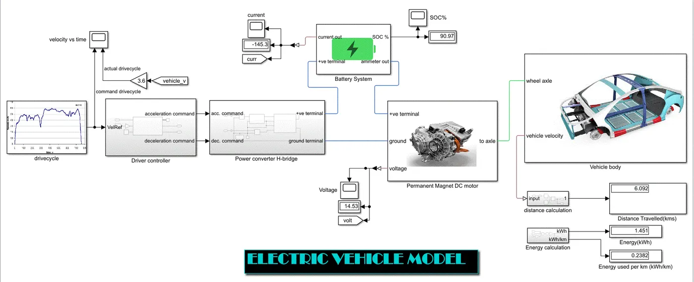
Above shown image is the developed model of electric car in MATLAB.

Vehicle:

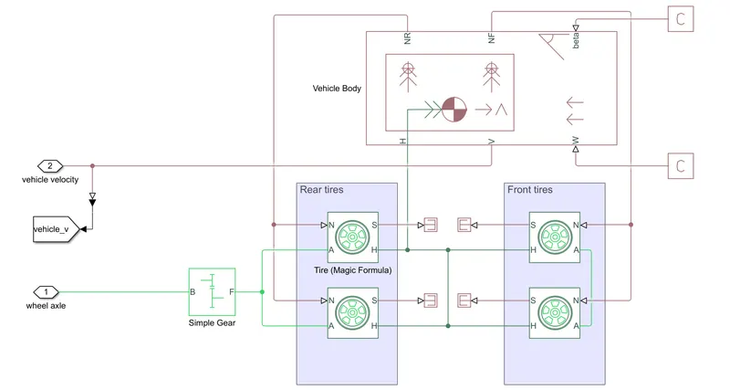
In this vehicle part it contains vehicle body, four tires,simple gear box.

• Vehicle body:

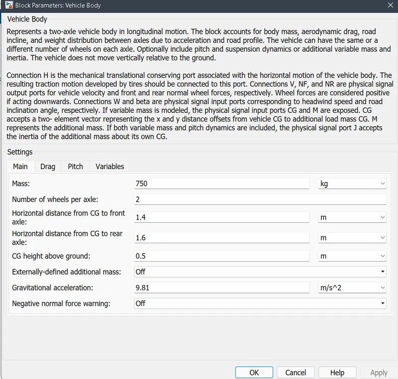
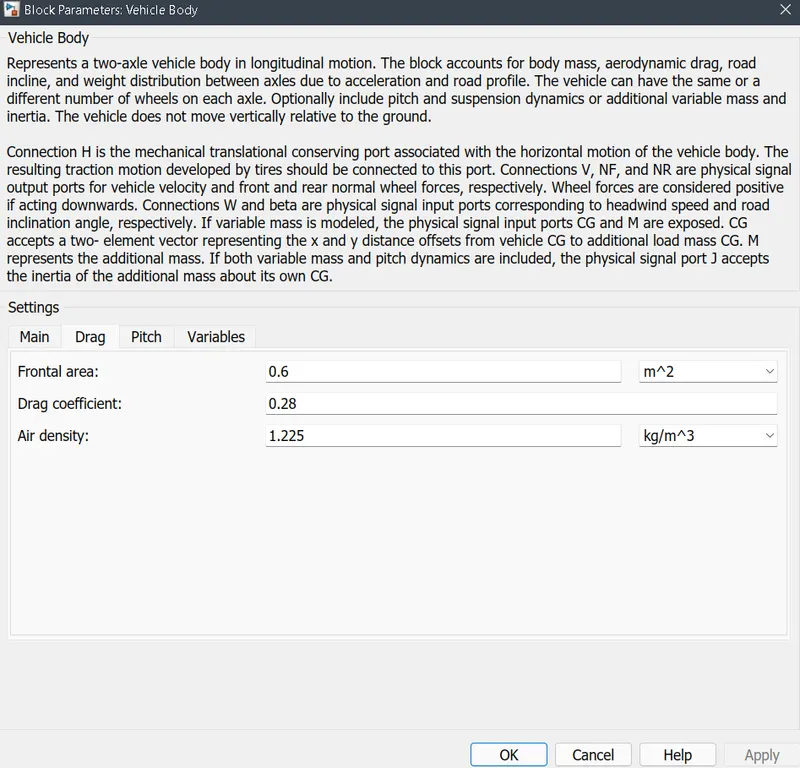
Represents a two-axle vehicle body in longitudinal motion. The block accounts for body mass, aerodynamic drag, road incline, and weight distribution between axles due to acceleration and road profile. The vehicle can have the same or a different number of wheels on each axle. Optionally include pitch and suspension dynamics or additional variable mass and inertia. The vehicle does not move vertically relative to the ground.Connection H is the mechanical translational conserving port associated with the horizontal motion of the vehicle body. The resulting traction motion developed by tires should be connected to this port. Connections V, NF, and NR are physical signal output ports for vehicle velocity and front and rear normal wheel forces, respectively. Wheel forces are considered positive if acting downwards. Connections W and beta are physical signal input ports corresponding to headwind speed and road inclination angle, respectively. If variable mass is modeled, the physical signal input ports CG and M are exposed. CG accepts a two- element vector representing the x and y distance offsets from vehicle CG to additional load mass CG. M represents the additional mass. If both variable mass and pitch dynamics are included, the physical signal port J accepts the inertia of the additional mass about its own CG.

The velocity of the vehicle os taken out from the 'V' port of the vehicle body.

Gradeability is given through Beta port and it is connected to a PS constant block where we can change the values

Wind velocity can be given through the W port and it is also connected to PS constant block

The values are specified below:

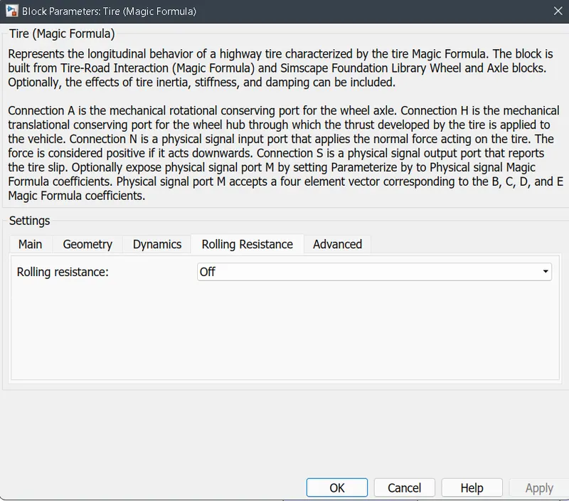
• Tire(Magic formula):

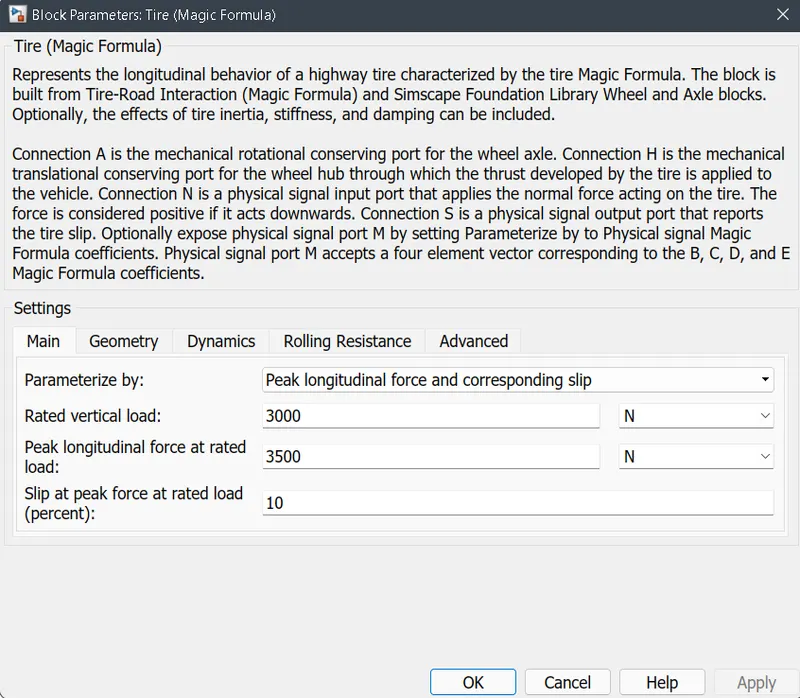
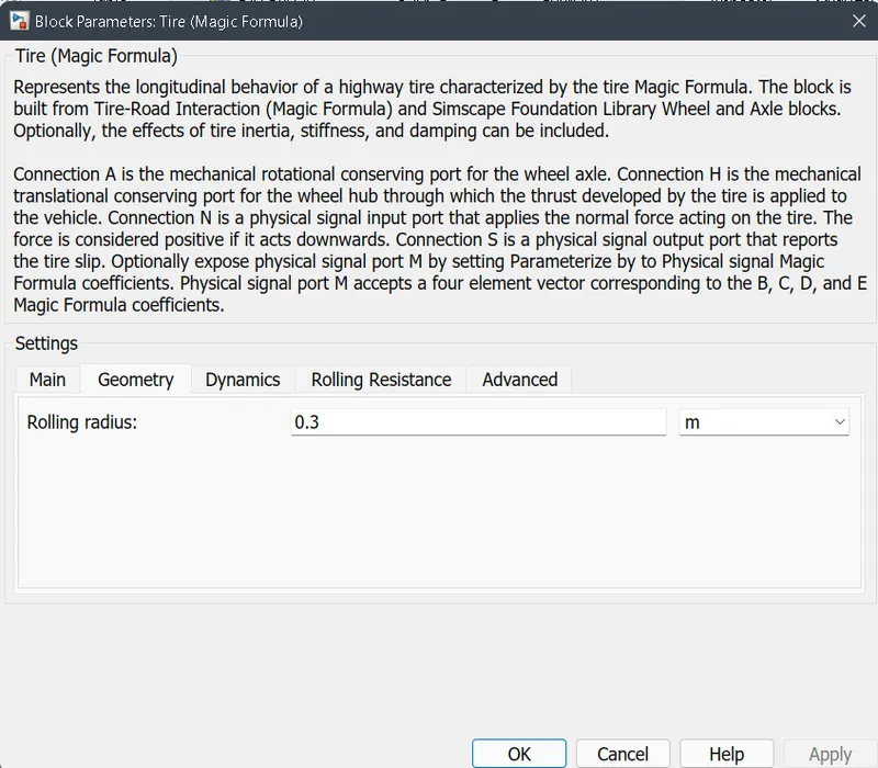
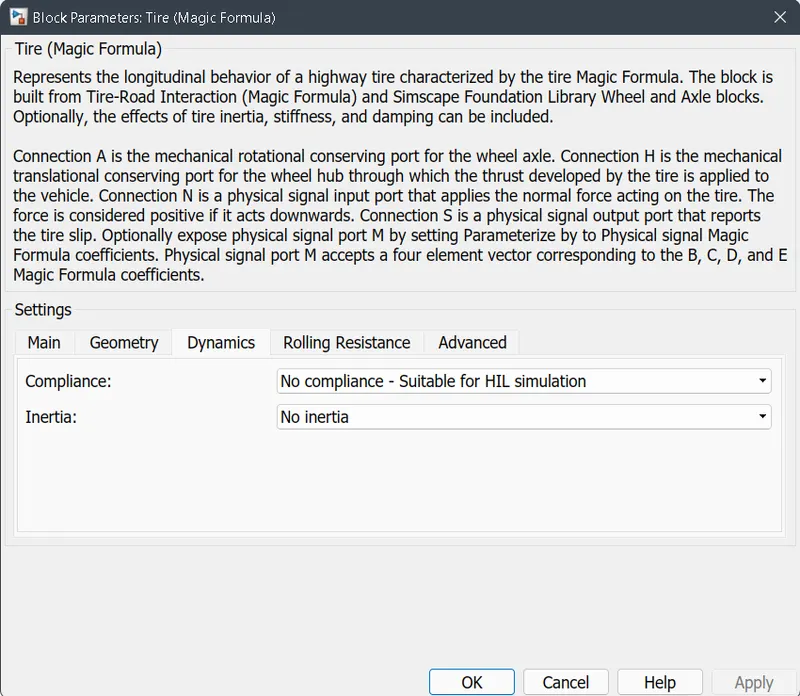
Represents the longitudinal behavior of a highway tire characterized by the tire Magic Formula. The block is built from Tire-Road Interaction (Magic Formula) and Simscape Foundation Library Wheel and Axle blocks. Optionally, the effects of tire inertia, stiffness, and damping can be included.Connection A is the mechanical rotational conserving port for the wheel axle. Connection H is the mechanical translational conserving port for the wheel hub through which the thrust developed by the tire is applied to the vehicle. Connection N is a physical signal input port that applies the normal force acting on the tire. The force is considered positive if it acts downwards. Connection S is a physical signal output port that reports the tire slip. Optionally expose physical signal port M by setting Parameterize by to Physical signal Magic Formula coefficients. Physical signal port M accepts a four element vector corresponding to the B, C, D, and E Magic Formula coefficients.

We have connected all the hub part of all 4 tires to the hub of the vehicle body.

Rear tires and Front tires are specified in the image

Normal force acting on the Tire is given through port 'N' and for rear tires N is connected to NR of vehicle body and for Front tires the 'N' is connected to the NF of electric vehicle body.

Here we are not giving any slip to the tires.The slip is given through S port.And it is terminated with terminator block.

Axle of front tires are connected each other

Axle of rear tires are connected to the simple gear box since it is a rear wheel drive

Here we are not giving any rolling resistance

The values entered are shown below:

• Simple gear:

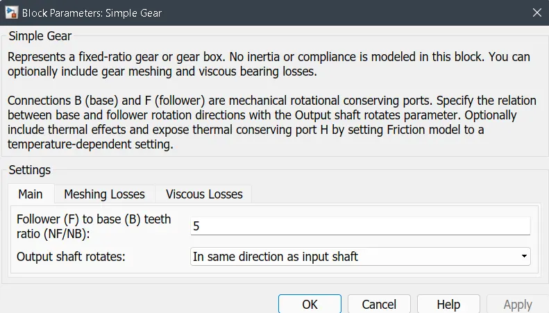
Represents a fixed-ratio gear or gear box. No inertia or compliance is modeled in this block. You can optionally include gear meshing and viscous bearing losses.Connections B (base) and F (follower) are mechanical rotational conserving ports. Specify the relation between base and follower rotation directions with the Output shaft rotates parameter. Optionally include thermal effects and expose thermal conserving port H by setting Friction model to a temperature-dependent setting.

Gear ratio here given is 5.

The output shaft rotates in the same direction as the input shaft.

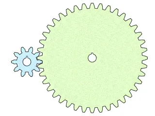
In the above shown figure the big gear is the follower and small one is Base.

follower output shaft is connected to the wheels inorder to increases theb torque and base is connected to the motor.

`Gear ratio,G = (Number of Follower teeth)/(Number of base teeth)`

Permanent Magnet DC motor:

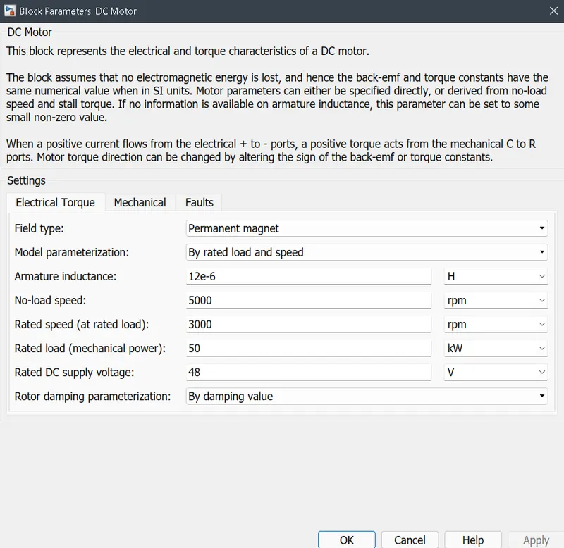
This block represents the electrical and torque characteristics of a DC motor.The block assumes that no electromagnetic energy is lost, and hence the back-emf and torque constants have the same numerical value when in SI units. Motor parameters can either be specified directly, or derived from no-load speed and stall torque. If no information is available on armature inductance, this parameter can be set to some small non-zero value.When a positive current flows from the electrical + to - ports, a positive torque acts from the mechanical C to R ports. Motor torque direction can be changed by altering the sign of the back-emf or torque constants.

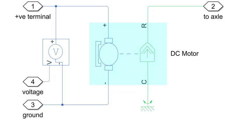
The armature of the motor is shown in blue color.The armature is given a voltage that is output of H-Bridge.This Voltage is measured using a voltmeter connected parallell to the motor.

The motor rated mechanical power is 50kW

The motor rated voltage is 48V DC supply

No load speed is selected as 5000rpm

At rated load the speed is 3000rpm

The C port is the casing where it is connected to the mechanical rotational reference.

The R port is the Rotary part it is connected to the simple gear transmission.

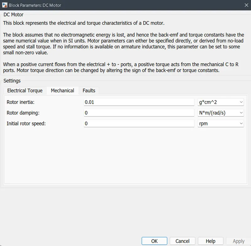
The selected values are specified below:

Battery system:

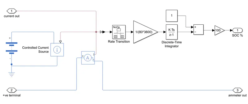
Battery system contains a battery having nominal voltage of 80V,a controlled current source,ammeter,rate transition block,gain blocks,dicrete time integrator,subtract block.

• Battery:

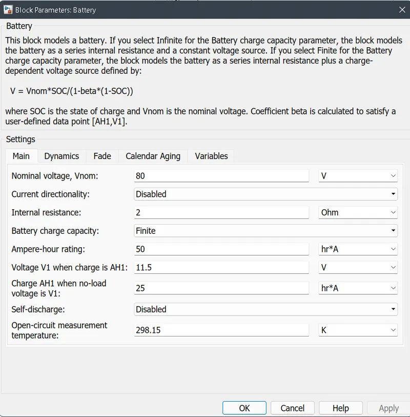
This block models a battery. If you select Infinite for the Battery charge capacity parameter, the block models the battery as a series internal resistance and a constant voltage source. If you select Finite for the Battery charge capacity parameter, the block models the battery as a series internal resistance plus a charge-dependent voltage source defined by:

V = `(Vnom*SOC)/(1-beta*(1-SOC))`

where SOC is the state of charge and Vnom is the nominal voltage. Coefficient `beta` is calculated to satisfy a user-defined data point [AH1,V1].

State of charge of a battery can be calculated as :

Here we are using a 80V,50Ah battery.

As the vehicle accelerates the battery gets discharged and when braking it gets charged beacuse of regenerative battery.

The battery specifications are shown below:

• Controlled Current source:

The block represents an ideal current source that is powerful enough to maintain the specified current through it regardless of the voltage across it. The output current is I = Is, where Is is the numerical value presented at the physical signal port.

It gives current that is given out by ammeter ,this current is from the H-bridge out.

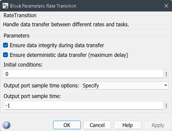
• Rate Transition:

This block is used to handle the data transfer between different rates and tasks.

• Gain block:

The output signal from the rate transition is multiplied by a gain value of `1/(80*3600)`

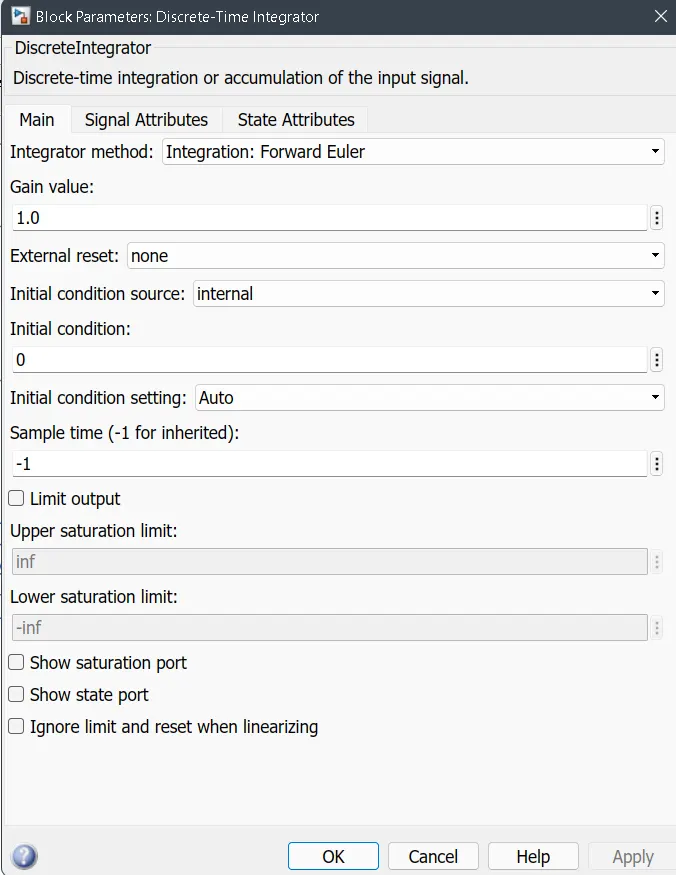
• Discrete Integrator:

This block is used for discrete time intregration or accumulation of the inputted signal.

This block outputs the amount of charge used by the battery.

And a subtracter block is used to subtract this value from the constant 1.

And this value is now multiplied with a gain of value 100.

Now this gain block outputs the State of Charge in %.

Power converter:

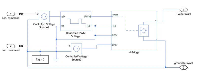
In this block there are two controlled voltage sources.

Controlled voltage source 1 receives the acceleration command from the driver controller.And a corresponding voltage is given to the controlled PWM voltage.

Also the controlled coltage source 2 receives the deceleration command from the driver controller.And this voltage is given to Brake input of H-bridge.

REV terminal of the H-bridge is connected to the reference terminal which provides the regenerative braking.

And according to the instructions given by the driver controller the controlled output voltage is outputted.

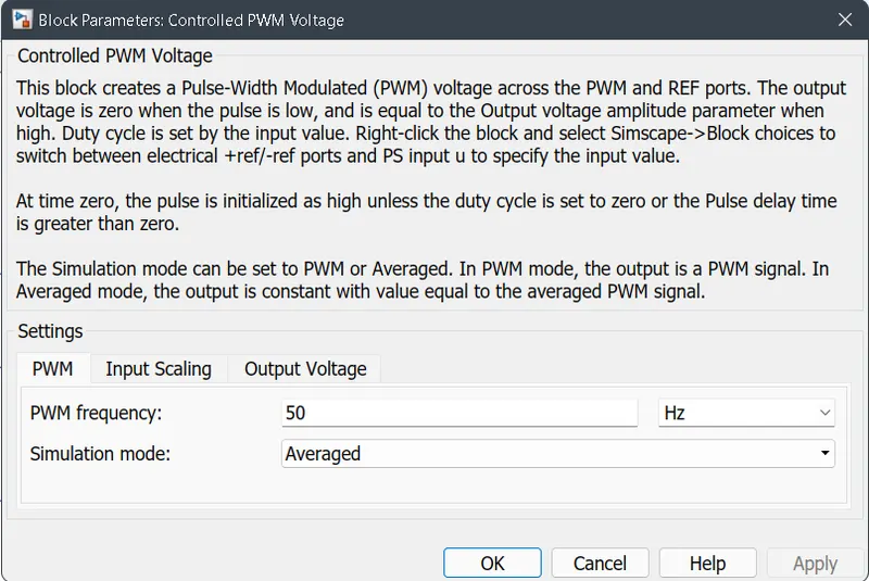
• Controlled PWM voltage:

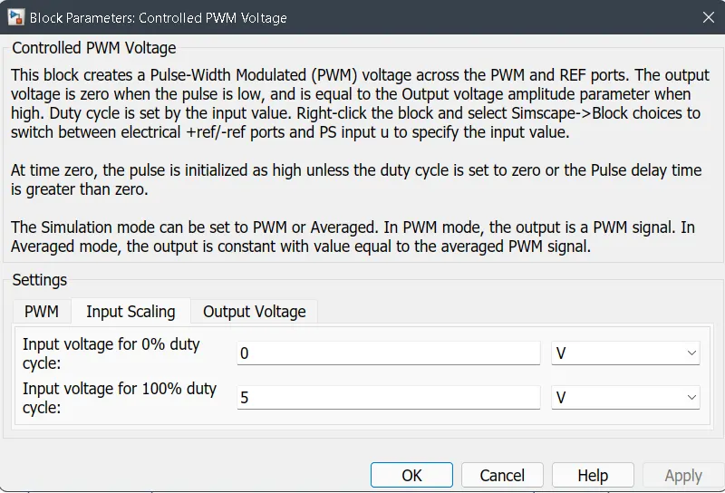
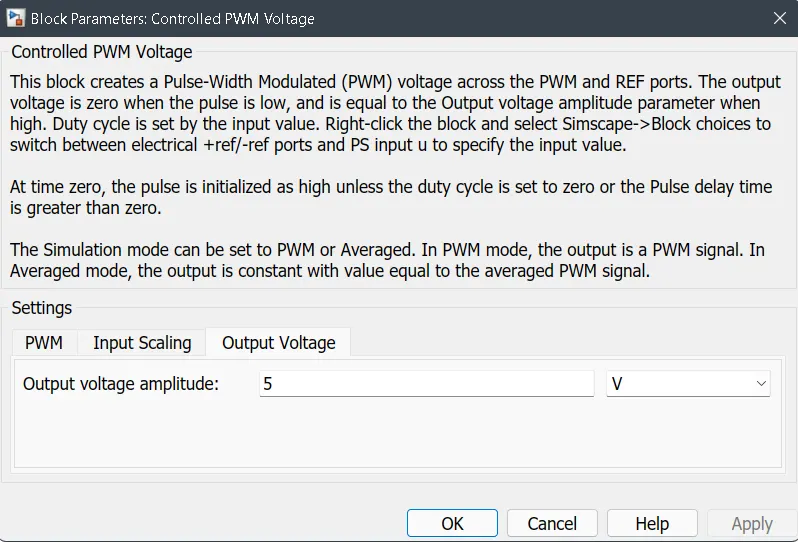
This block creates a Pulse-Width Modulated (PWM) voltage across the PWM and REF ports. The output voltage is zero when the pulse is low, and is equal to the Output voltage amplitude parameter when high. Duty cycle is set by the input value. Right-click the block and select Simscape->Block choices to switch between electrical +ref/-ref ports and PS input u to specify the input value.At time zero, the pulse is initialized as high unless the duty cycle is set to zero or the Pulse delay time is greater than zero.The Simulation mode can be set to PWM or Averaged. In PWM mode, the output is a PWM signal. In Averaged mode, the output is constant with value equal to the averaged PWM signal.

The specified values are shown below:

• H-Bridge:

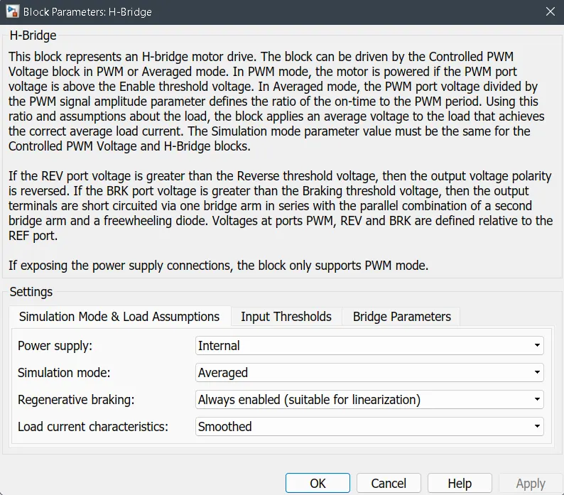
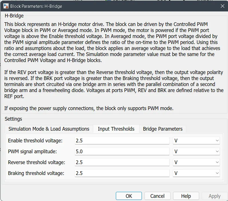
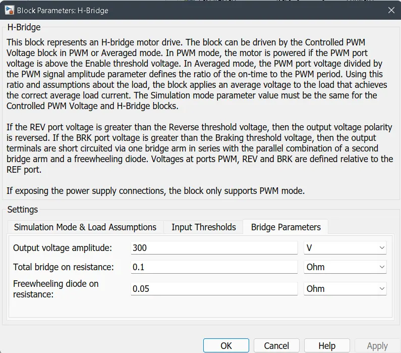
This block represents an H-bridge motor drive. The block can be driven by the Controlled PWM Voltage block in PWM or Averaged mode. In PWM mode, the motor is powered if the PWM port voltage is above the Enable threshold voltage. In Averaged mode, the PWM port voltage divided by the PWM signal amplitude parameter defines the ratio of the on-time to the PWM period. Using this ratio and assumptions about the load, the block applies an average voltage to the load that achieves the correct average load current. The Simulation mode parameter value must be the same for the Controlled PWM Voltage and H-Bridge blocks.If the REV port voltage is greater than the Reverse threshold voltage, then the output voltage polarity is reversed. If the BRK port voltage is greater than the Braking threshold voltage, then the output terminals are short circuited via one bridge arm in series with the parallel combination of a second bridge arm and a freewheeling diode. Voltages at ports PWM, REV and BRK are defined relative to the REF port.If exposing the power supply connections, the block only supports PWM mode.

The regenerative braking option is enabled

The simulation time is averaged otherwise simulation takes more time

The output voltage amplitude is 300V

The specified values are given below:

• Driver controller

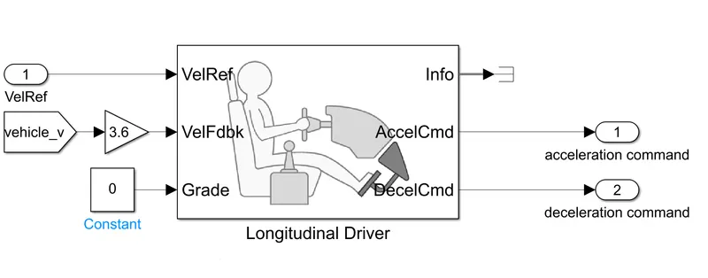
• Longitudinal driver:

A parametric longitudinal speed tracking controller for generating normalized acceleration and braking commands based on reference and feedback velocities.Use the external actions to input signals that can disable, hold, or override the closed-loop commands determined by the block. The block uses this priority for the input commands: disable, hold, override.

Longitudinal driver simply gives acceleration and deceleration commands according the drive cycle data.

The velocity data extracted from the drive cycle is given here as a velocity reference.

The velocity from the vehicle body is taken and it is fedback to this block.

The gain 3.6 is nothing but converting velocity in m/s to km/hr.

Here we can give the gradeability as well through a constant block.

According to the drive cycle the driver gives the acceleration and deceleration command to the power converter block.

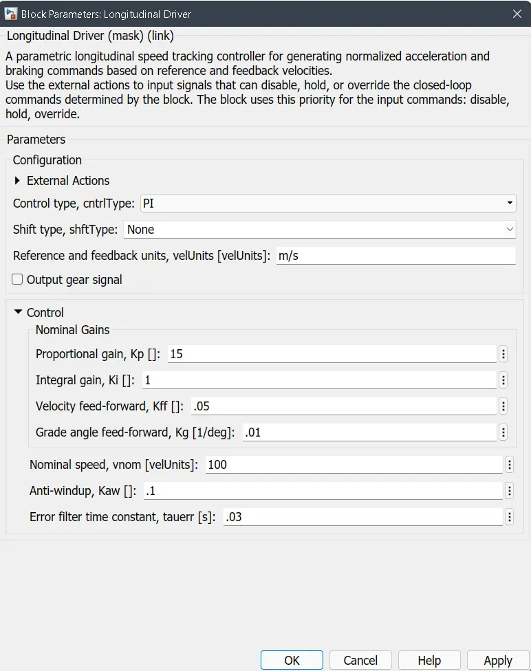
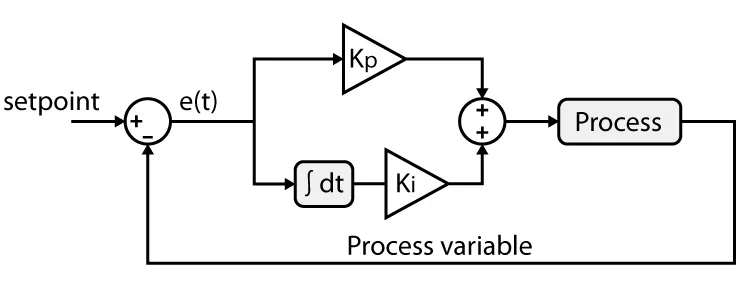
In this longitudinal driver model Proportional Integrator Type controller is used.

Energy consumed and distance calculation:

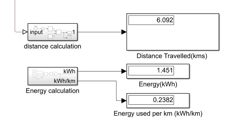
Distance calculation:

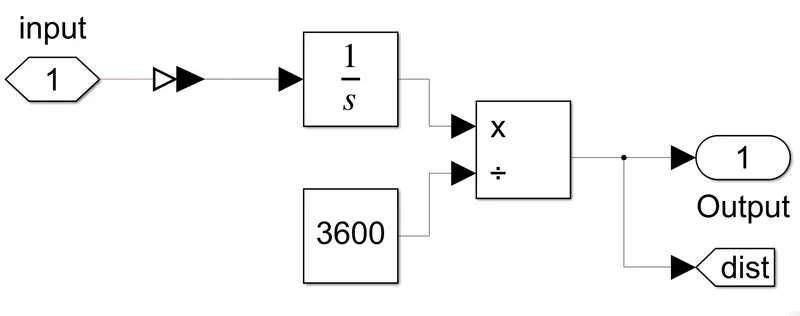
The total distance travelled is calculated by taking the velocity and integrating using integrator block and dividing this value by 3600 to give the result in kilometres.

Energy calculation:

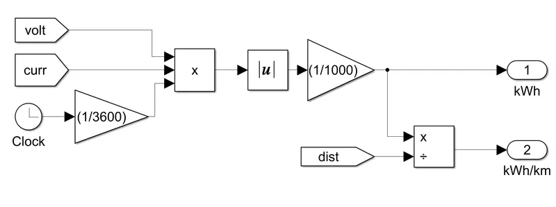
Energy is calculated using the equation :

Energy = Voltage * current * Time

Energy consumed per kilometre is calculated simply dividing Energy by total distance covered.

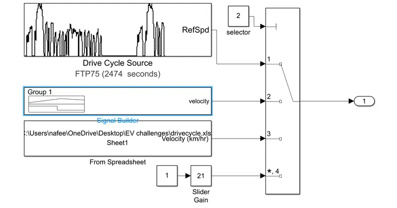
Drivecycle:

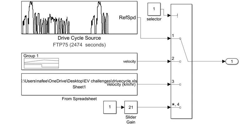
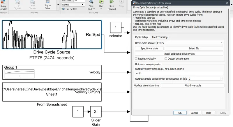
This drive cycle block has four different drive cycle sources.They are:

1. FTP75
2. Signal builder source
3. From spreadsheet
4. Using slider gain as an accelerator

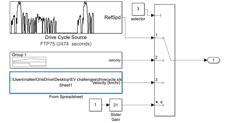
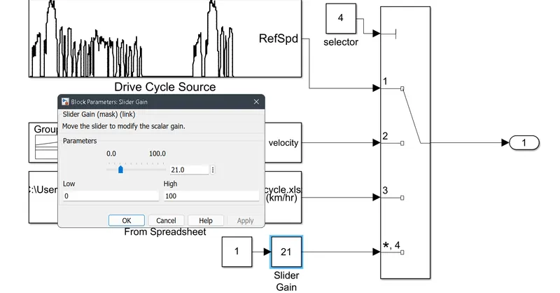
we can select the drive cycle source by simply assigning the values 1,2,3,4 in multiport switch selector that is the constant block.

Case 1:

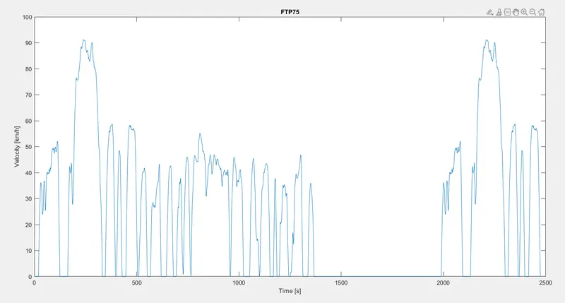
The drive cycle given here is using the Drive cycle source block in Simulink.In that they have many option I selected 'FTP75' which is a predefined drive cycle which has aduration of 2474 seconds.We can select this drive cycle option by simply assigning value '1' in the multiport switch selector.And the FTP75 drive cycle is outputted.

The drive cycle FTP75 plot:

These are the calculated values:

The ouput plots:

1. Drivecycle plot

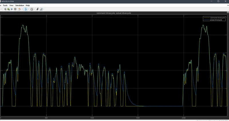
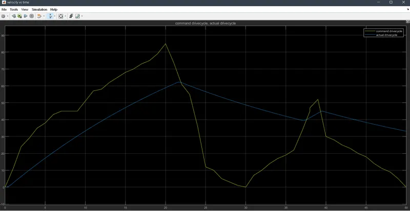
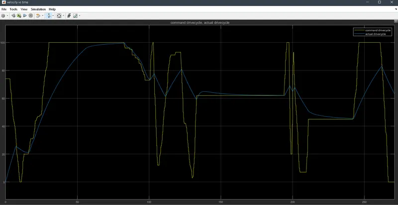
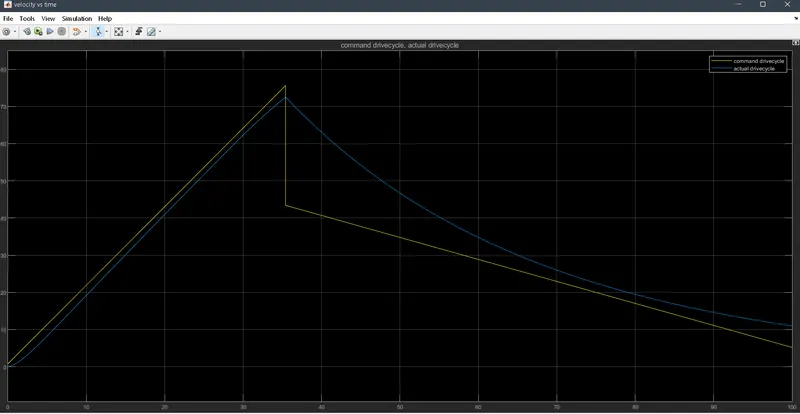
Here we can see the drive cycle of both the command drivecycle and the actual drive cycle.Blue is actual and yellow is command drive cycle.

We can see the closeness of both drivecycles it is intersecting with each other.

The increase in velocity means it is accelerating and decrease in velocity means it is decelerating.

2. The voltage plot

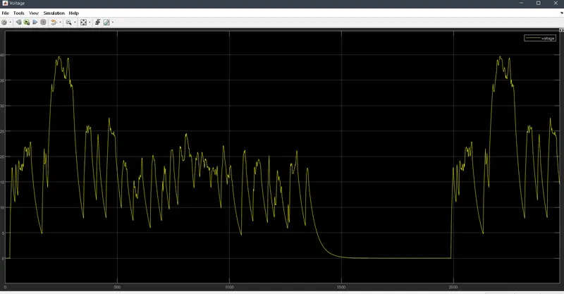
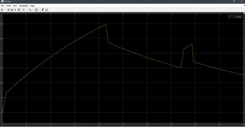
Here we can see the volatge increases and decreases according the drive cycle.

When velocity is high more voltage also increases.

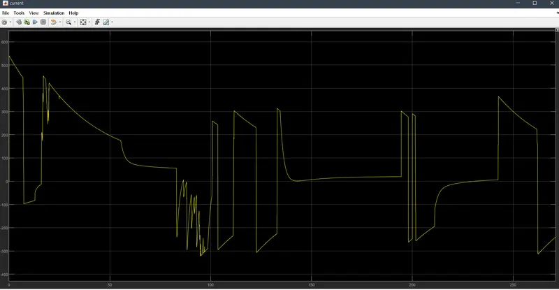
3. Current plot:

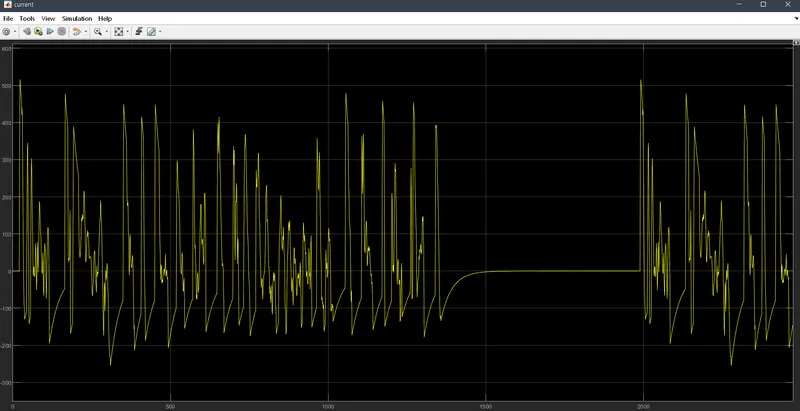
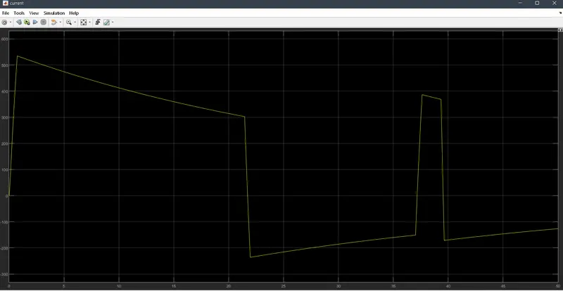
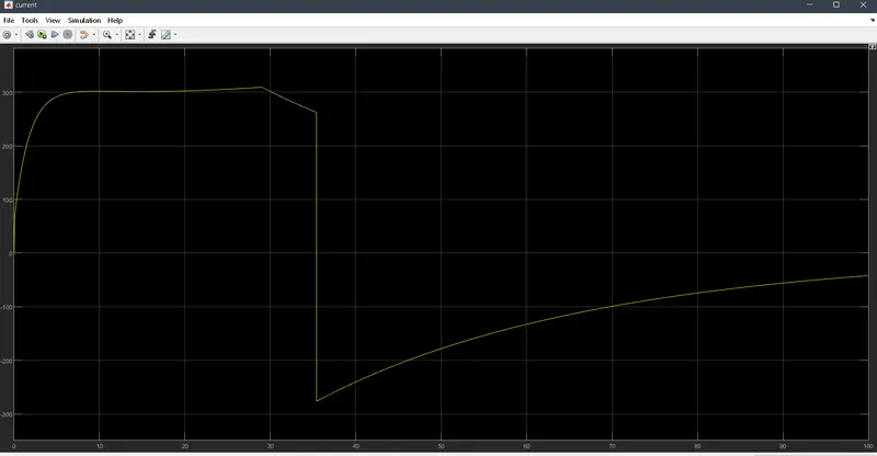
The current is first increasing when the vehicle accelerates when decelerating because of regenerative braking current flows reverse to the battery.

When braking the motor acts as generator.

At last the current is negative it means that the battery is charging.

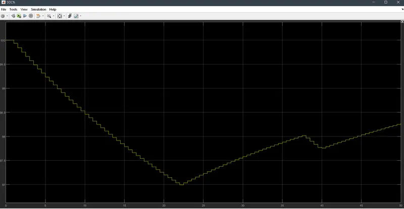
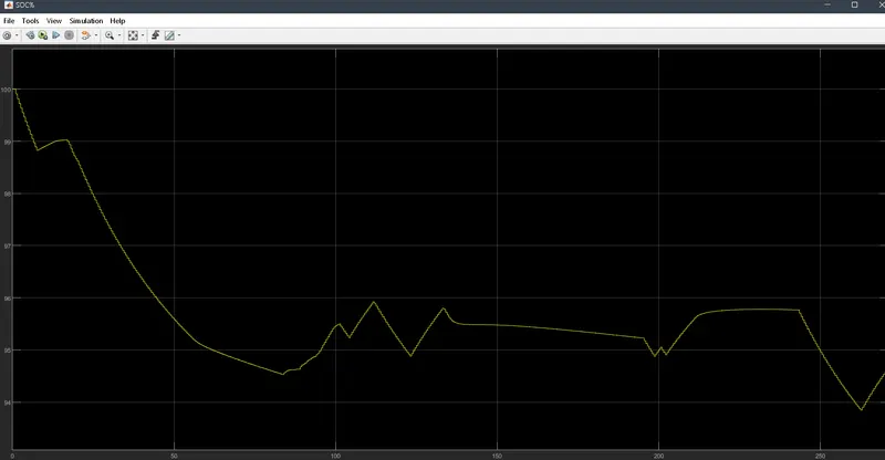
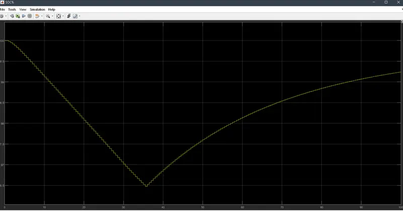
4.The SOC plot:

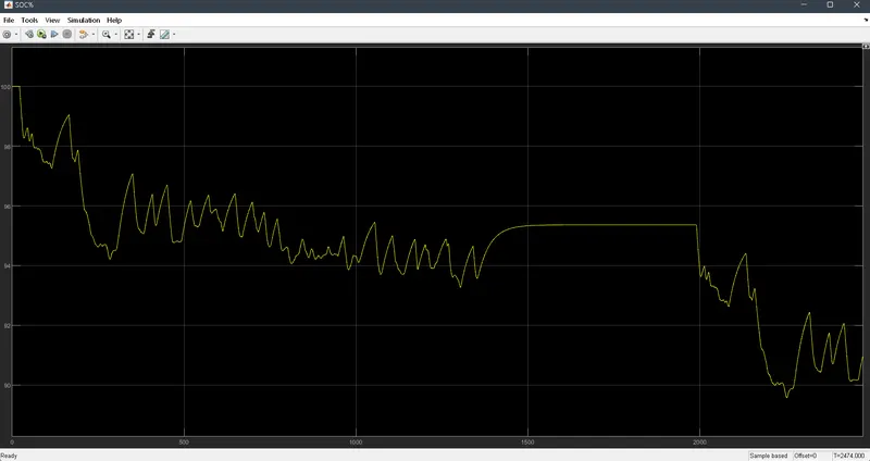
The state of charge is the measure of how much charge is left inside the battery.

At the beginning the SOC is 100% and when vehicle accelerates the SOC is dropping because as the current drawn from the battery increases the battery discharges.

As the vehicle is braking or decelerating the SOC increases because due to regenerative braking the battery is getting charged ,so SOC increases.

SOC remains constant when there is no acceleration or braking.

Case 2:

The drive cycle given here is using a block called From spreadsheet.In the excel sheet I have created data containing velocity and time.This file named 'Mydrivecycle.xlsc' is given to the from spreadsheet block.And this drive cycle is outputted.This can be selected by simply assigning the value '3' in multiport switch selector.

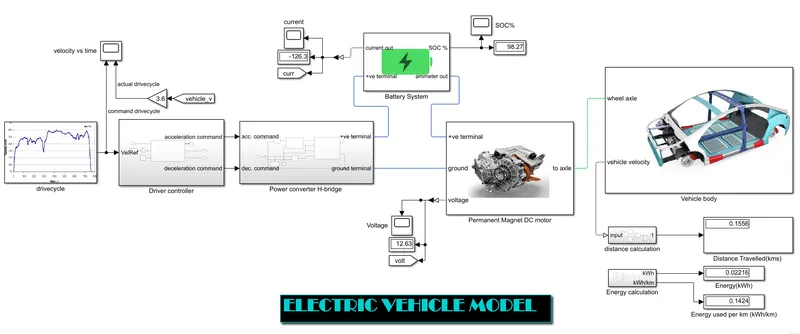
1.The drive cycle plot:

2. The voltage plot

3. Current plot:

4.The SOC plot:

Case 3:

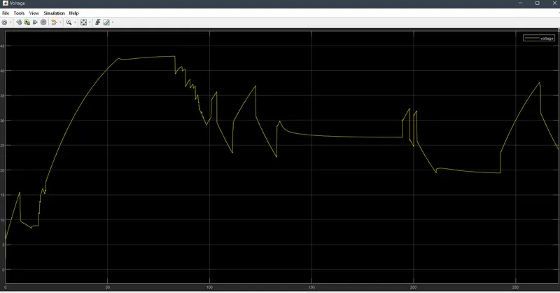
The drive cycle source here we are giving is through a simple slider gain block used as an accelerator.The simulation time is 300 sec.It is given by assigning the value '4' in multiport switch selector and the output will be slider gain output.By adjusting the slider we can accelerate or decelerate the vehicle according to our need.

1. Drivecycle plot

2. The voltage plot

4.The SOC plot:

3. Current plot:

Case 4:

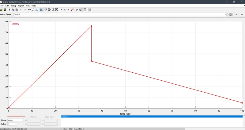
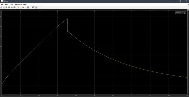
The drive cycle source given here is by using a signal builder block.The velocity in y-axis and time in x-axis is built in a signal builder block.The signal builder block is selected just by assigning the value 2 in the multiport switch selector.The built signal is shown below:

1. Drivecycle plot

3. Current plot:

2. The voltage plot

4.The SOC plot:

Result Table:

Vehicle parameters	Case 1	Case 2	Case 3	Case 4
Drive cycle Duration Distance Top speed	FTP75 2474 sec 6.092 kms 91.46 km/h	From spreadsheet 50 sec 0.1556 km 62.23 km/h	Slider gain 300 sec 1.367km 100km/h	Signal builder 100 sec 0.2586 km 75 km/h
Vehicle weight	750 kg	750 kg	750 kg	750 kg
Frontal area drag coefficient Rolling resistance	0.6 `m^2` 0.28 0	0.6`m^2` 0.28 0	0.6`m^2` 0.28 0	0.6`m^2` 0.28 0
SOC at end of drive cycle (Initial OSC 100%)	90.97%	98.27%	94.67%	99.24%
Energy used kWh per km	1.451 kWh 0.2382 kWh/km	0.02216 kWh 0.1424 kWh/km	0.4372 kWh 0.3198 kWh/km	0.004896 kWh 0.01893 kWh/km

Comments on results:

• Power rating of DC motor and maximum vehicle speed
• PI control loop gains for tracking reference speed
• Battery discharge and km per full charge
• Regenerative braking effect
• Various model library (simscape,simulink, and powertrain blockset) categories
• Simulation time and drive cycle time

Conclusion:

MATLAB model of a simple,low runtime electric car is designed by using battery,DC motor.It is simulated and the results are plotted and it is verified.The performance changes for different parameters and configurations are studied.The changes in results for various drive cycles are understood.Checked various parameters like Voltage,Current,SOC,Velocity for different conditions.