Final Project: Design of an Electric Vehicle

                                                                               Final Project On Design Of An Electric Vehicle With Matlab-Simulink.

Create a MATLAB model of electric car which uses a battery and a DC motor. Choose suitable blocks from Powertrain block set. Prepare a report about your model including following:

Objectives: 

       1. System level configurations

       2. Model parameters

       3. Results

       4. Conclusion

Electric Vehicle (EV) :-

An electric vehicle (EV) is a vehicle that uses one or more electric motors or traction motors for propulsion. An electric vehicle may be powered through a collector system by electricity from off-vehicle sources or may be self-contained with a battery, solar panels, fuel cells or an electric generator to convert fuel to electricity. EVs include, but are not limited to, road and rail vehicles, surface and underwater vessels, electric aircraft and electric spacecraft.

                            

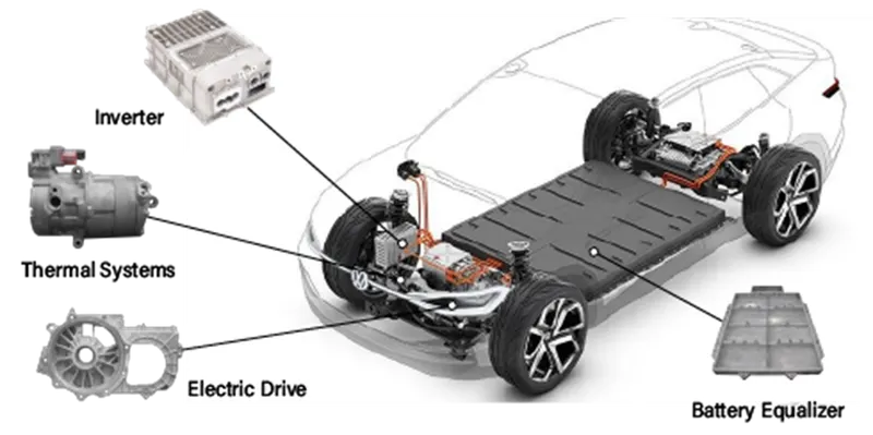
EVs first came into existence in the mid-19th century, when electricity was among the preferred methods for motor vehicle propulsion, providing a level of comfort and ease of operation that could not be achieved by the gasoline cars of the time. Internal combustion engines were the dominant propulsion method for cars and trucks for about 100 years, but electric power remained commonplace in other vehicle types, such as trains and smaller vehicles of all types.

Commonly, the term EV is used to refer to an electric car. In the 21st century, EVs have seen a resurgence due to technological developments, and an increased focus on renewable energy and the potential reduction of transportation's impact on climate change and other environmental issues. Project Drawdown describes electric vehicles as one of the 100 best contemporary solutions for addressing climate change.

component of the electrical vehicle :

                                            

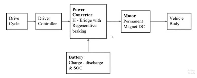
                                                              FIG.BASIC BLOCK DIAGRAM OF ELECTRIC VEHICLE.

the vehicle body mainly consists of ,

1.  vehicle body
2.  motor & converter
3. battery Bank & power converter 
4. standard drive cycle source.

simulink model:-

shown below is the simulink model of the electric vehicle 

                                

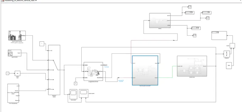
Detailed Model Study : parameter & configuration

1) VEHICLE BLOCK:

the vehicle block consists of tire,  body of tire, transmission of energy. block shown below.

                     

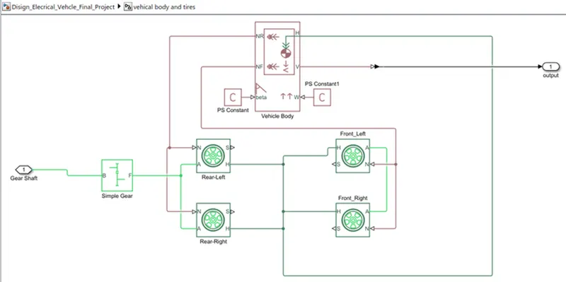
vehicle body:

the above simulink model show the vehicle body along with rear and front wheel and simple gear is attached to the wheel.

                                                 

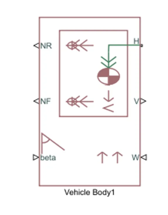
o Input Ports:

W=Wind Velocity in m/s

beta=Grade angle in radians                                                    

o Output Ports:

V=Velocity in m/s

NR=Normal force on Rear Axle (N)

NF=Normal Force on Front Axle (N)

                                                      

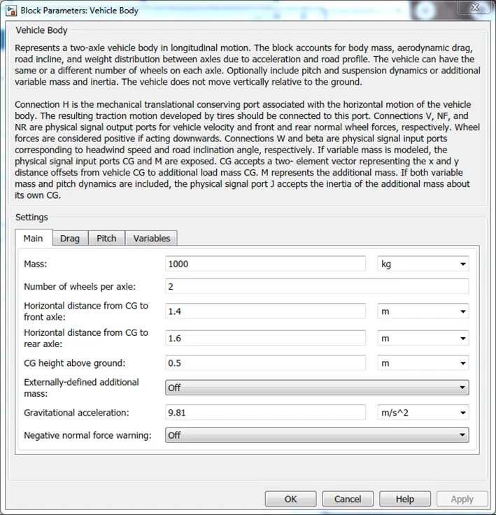
the mass of the vehicle is varied i.e 1000kg in main section, pitch section is kept ON ,In drag and variable section we kept default value .

 tire:

                                                           

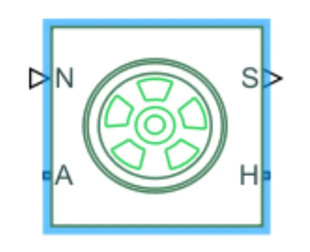
The vehicle is assumed to be front axle is driven (4 wheels- 2 on each axle).

The wheels are modelled using simple Tire (Magic formula) Simulink blocks.

The block can model tire dynamics under constant or variable contact surface

conditions.

• Input Port:

N=Normal force acting on the tire, positive when force is acting downwards/towards the contact surface.

• Output Port:

S=Slip value is relative to tire and surface of contact.

• Conserving Ports:

H=represents wheel hub which transmits thrust generated by the wheel to the body of the vehicle.

A=represents the axle on which the tires are mounted

tire parameter:

                                                 

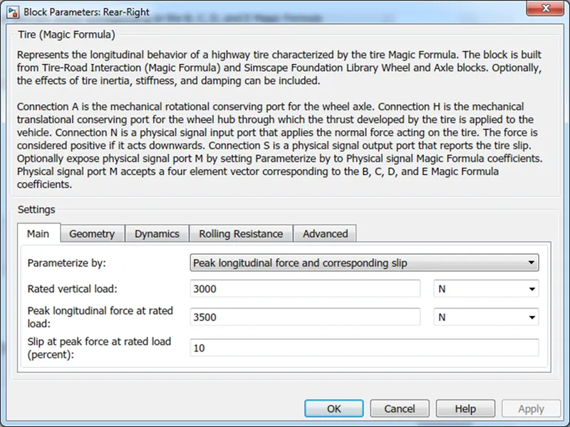
• The tires are parameterized by Peak longitudinal force and corresponding slip
• The other block parameters such as rated vertical load, peak longitudinal force at rated load and slip at peak force at rated load - are kept with their default values.

Gear:

                                       

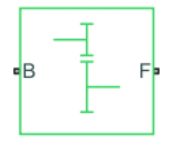
A simple gear block is used to connect the motor to the rear axle of the vehicle.

It represents the gearbox that connects the input shaft to the base gear and output from the follower gear.

Conserving Ports:

B=port associated with an input shaft (motor shaft)

F=port associated with the output shaft (axle/ differential)

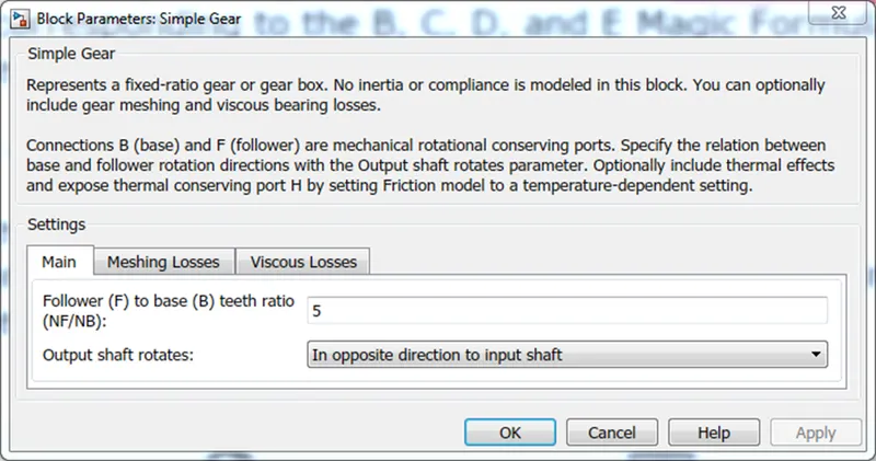
Simple Gear Parameters:

Gear ratio and output direction are modified. Meshing loss is kept constant and gear is having a constant efficiency throughout the simulation.

Viscous losses and faults are kept at default conditions.

                                                      

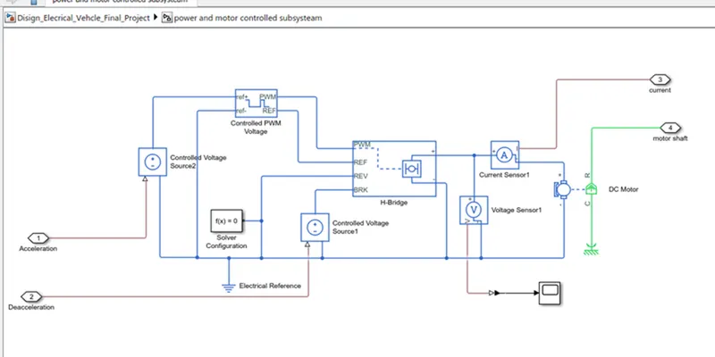
2) motor & power converter :

these block consists of controlled PWM voltage ; H-bridge & DCmotor

                         

H-Bridge:-

the H-bridge is an electronic circuit that switches the polarity of a voltage applied to the load. and allow DC motor to run forward and backward.

                       

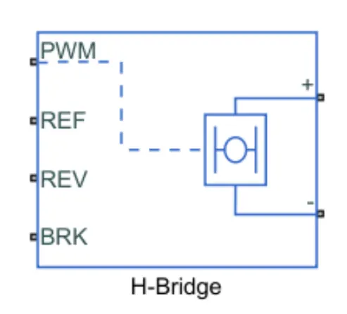
The H-Bridge helps in controlling the power that is input according to the requirement. The output provided is converted voltage as per the controlled parameters.

                         

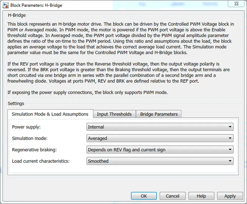
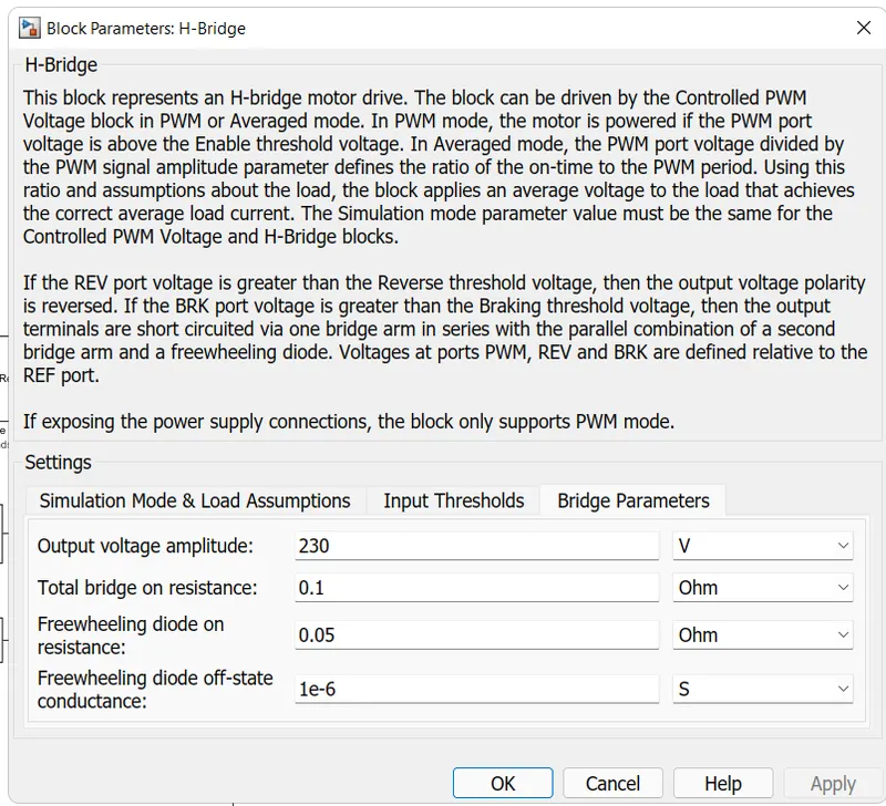
• H-bridge has its own internal source
• averaged simulation mode is selected for faster simulation and regenerative is enabled
• load characteristics are kept smoothed 
• in bridge parameter output voltage is kept as a rated votage of a motor. remaining value set as default.

D.C Motor:-

                          

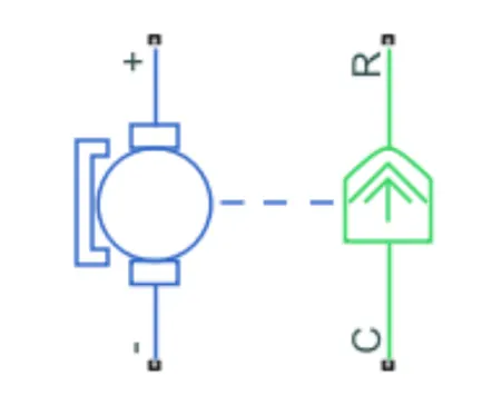
This is the DC Motor which would give rotational power to the wheels and become the sole power generation source.

The DC Motors terminals are connected as mentioned below.

+ =Electrical signal to the motor Positive Terminal

- =Electrical signal to the motor Negative Terminal

R=Casing of the Motor connected with the Mechanical Rotational Reference Block

C=Rotor Case connected to the Mechanical Rotational reference.

                           

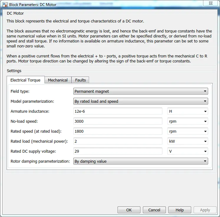
The parameter considered is, The Armature inductance is as default, varied the changes in the No-Load Speed 3000 rpm, the rated speed 1500 rpm, the Rated Load at 50kW, and the Rated DC Supply Voltage 230 V. All other parameters are as default.

Controlled PWM Voltage;

                             

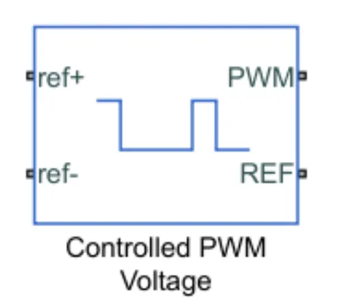
The Controlled PWM Voltage Block helps in keeping the Modulated Pulses as per the required pulses. So that the operations happen smooth and higher variations are not observed.

The Ports are connected as follows.

PWM=PWM connected directly to the H-Block

REF=REF connected directly to the H-Block

ref+ = Reference Positive connected with Driver Model ith the Acceleration Commands from the

ref- =Reference Negative connected with the Deceleration Commands from the Driver Model

Note: The parameters are set as default.

                    

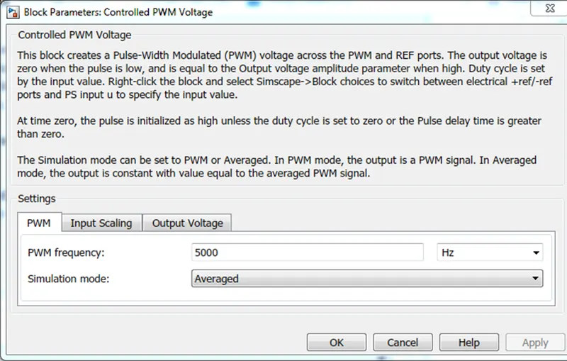
according to the need of the accuracy the simulation should be run in the PWM mode which consume time but good in the acccuracy;

while in the averaged mode the accuracy is less 

3 Battery and SOC System:-

                     

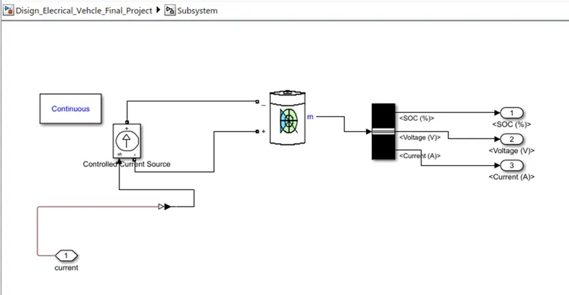
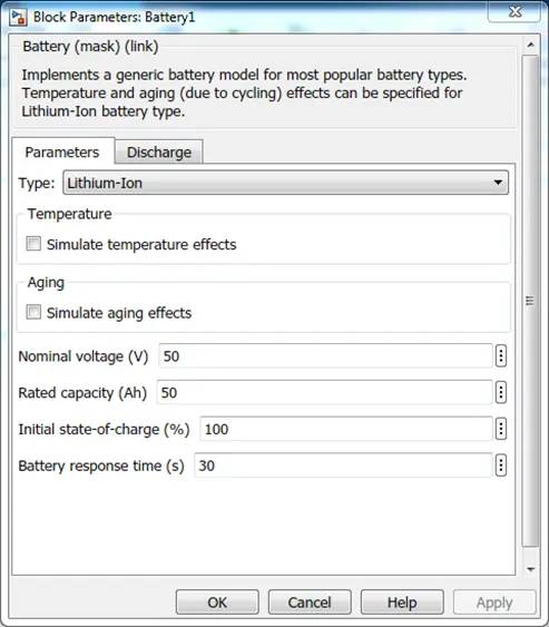
 Battery:-

• Most electric vehicles use lithium-ion batteries (Li-Ions or LIBs). Lithium-ion batteries have a higher energy density, longer life span and higher power density than most other practical batteries. Complicating factors include safety, durability, thermal breakdown and cost. Li-ion batteries should be used within the safe temperature and voltage ranges in order to operate safely and efficiently.
• The prices of lithium-ion batteries are constantly decreasing, contributing to a reduction in the price of electric vehicles.

                                       

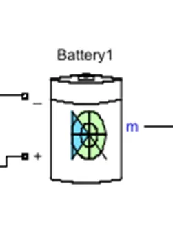
Implements a generic battery model for most popular battery types. Temperature and ageing (due to cycling) effects can be specified for Lithium-Ion battery type.

                              

controlled Current Source:- 

                               

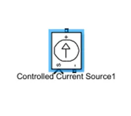
a controlled current source is connected to the lithium battery. this controlled current source provided will initiate the flow of current from the battery to the motor and during regenerative braking from the motor to the battery. the acceleration and deacceleration is provided through controlled current source ; while acceleration current demand is  high  while at deacceleration i.e braking energy stored called regnerative braking in the battery.

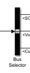
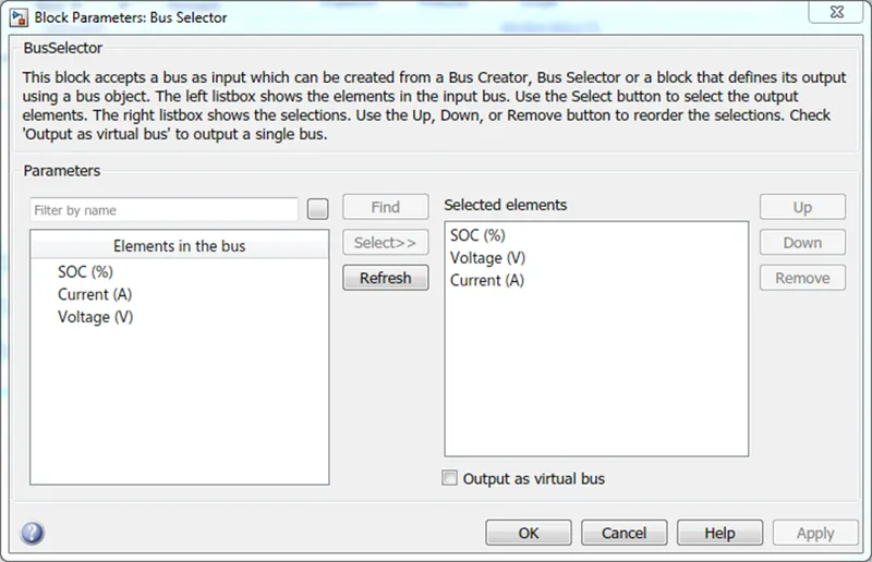
Bus selector : 

the number of output is selected through the bus selector in our simulation there are 3 output port 1)%soc 2)voltage 3) current.

                                          

               

4 Longitudinal Driver:-

                      

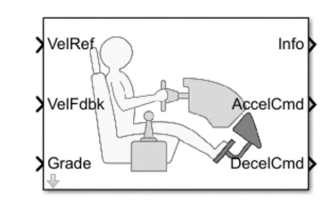
It is a parametric longitudinal speed tracking controller for generating normalized Acceleration and Braking commands based on reference and feedback velocities,

• The VelFdbk port corresponds to the feedback velocity. The actual velocity output given by the vehicle body is connected here. By comparing the actual (feedback) velocity with the reference velocity, the driver block generates acceleration and braking signals in order to minimise the error between the two concerned velocities.
• Grade corresponds to the grade angle. For this simulation, no inclination is considered and hence, a constant block with value 0 is connected.
• Info gives the output for the bus signal for different block calculations like the difference in reference vehicle speed and vehicle speed, etc.
• AccelCmd & DecelCmd correspond to the acceleration and deceleration commands generated respectively and are connected to the corresponding ports of the Controlled PWM Voltage block Here, the selected control type is Pl. Accordingly, the block implements proportional-integral (PI) control with tracking windup and feed-forward gains.

                       

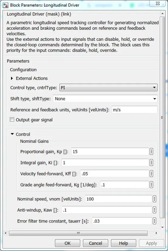
represent the longitudinal speed controller which produce acceleration  & deacceleration  based on the command input and feedback speed variable

providing using a proportonal integral (PI)

5 Reference Velocity (Drive Cycle):

• The Drive Cycle Source block is used to provide the reference speed for the simulation.
• It generates a standard or user-specified longitudinal drive cycle.
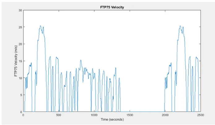
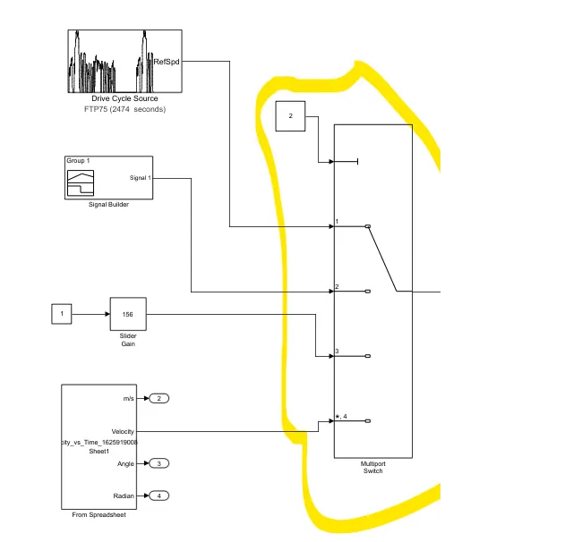
• BY DEFAULT FTP75 is selected there are also slider gain ,signal block, spreadsheet ,WOT(wide open throttle). etc.
• default time fopr simulation is 2474.

                         

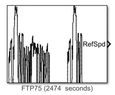
The no's of standard drive are present like UDDS but as default we use FTP 75  

                              

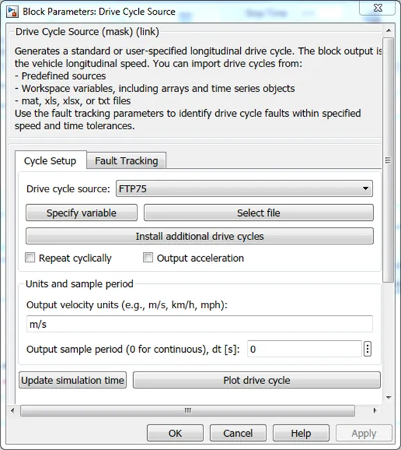
the below shown is the VELOCITY VS TIME(SEC) graph of drive cycle FTP75 (FEDERAL TEST PROCEDURE).

                                   

 6) Distance in km/hr:-

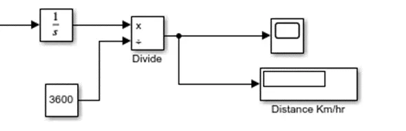
The scope will display velocity of the vehicle in km/hr to measure the distance in km, an integrator block is used because the interaction of velocity will give us distance and 3600 constant blocks are used because 1hr=3600sec

                                     

7) MULTIPORT SWITCH:- 

 the below highlight is a multiport switch the 4 no,s of different input is given  the constant block connected to multiport switch

help to select specified input now the constant number is displayed is 2 as we see in below that means signal builder input is connected to the further simulation 

of the vehicle from the 4 input. 

                                                     

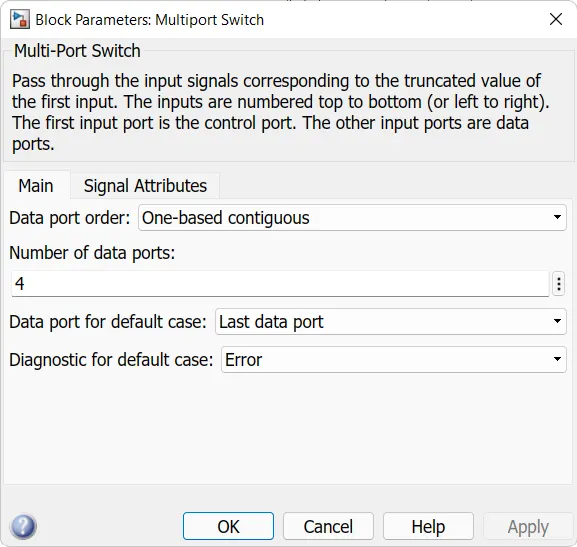
from the multiport switch block parameterwe can select the number of data port remaining we kept as a default.

8 Simulink Explanation:-

The system is running for simulation for 1080s which is the total time for which the input drive cycle is defined.

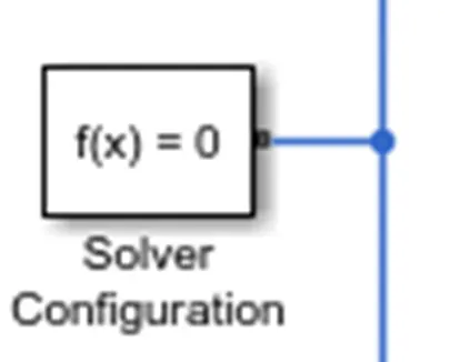
A Solver Configuration is added to ensure proper solving of the mathematical equations by the model.

                                   

• Scopes are connected to analyze different outputs such as the SOC of the battery, the reference velocity & the actual velocity of the vehicle and the distance covered by the vehicle during the total run

result:-

               

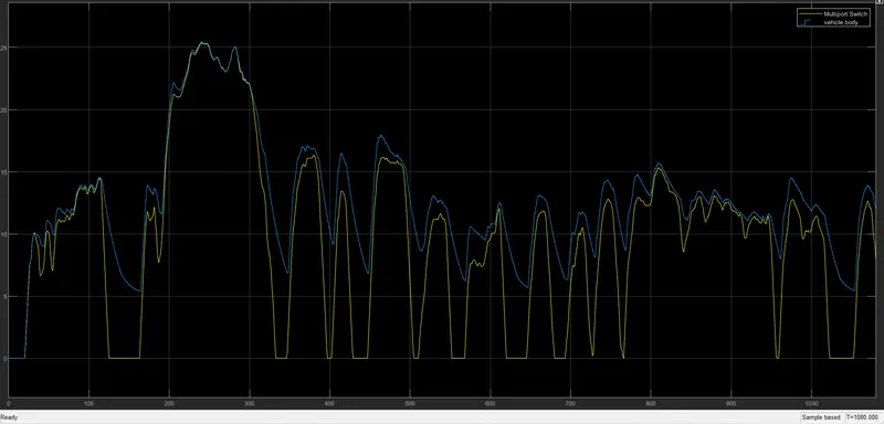
The blue line is a graph of the vehicle speed source and the yellow line shows the corresponding drive cycle graph(actual velocity)

both the graph do not follow the each other due to the actual vehicle speed is different than drive cycle. but there is not drastacally change in the graph 

the PWM  simulation mode will give much accurate graph than the averaged one 

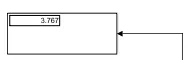
the above simulation take 1080

sec to travelled the 3.767km distance.

                                           

SOC calculation:-

the below graph shows the change in SOC

                 

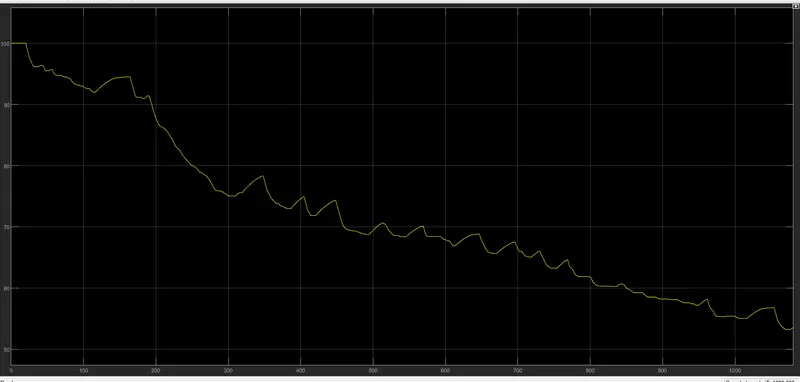
the state of charge goes on decreasing from 100% to 53.53% i.e 50 % battery get discharge to travelled the distance of 3.767km in 30 min approx.

hence from these graph we can know the remaining capacity of the battery.

the change of battery voltage is given below.

              

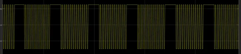
the voltage appeared in display box is 55.41v so that to travelled the distance of 3.767km battery takes the 55.41v 

the change of battery current is given below

           

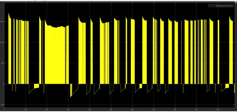
in above graph at the time of braking we can see the extra current generated is moving to charge the battery  

conclusion:-

the detailed and in depth parameterizationof the motor control and vehicle block variable would make the model to exactly follow the reference velocity signal 

modification in battery block variable might be helpful to increases the performance of depth of discharge 

and last, to traveled the distance of 3.767 KM  it take 1080 sec to simulate and 50% discharge of battery.

FUTURE SCOPE:-

• optimization of battery pack for increasing mileage and peak performance 
• detailed simulation rather than performing averaged mode simulation
• to reduce the variation between reference speed signal and actual speed signal.

ATTACHMENT : 2 NUMBER

THE BLOCK DIAGRAM OF ELECTRIC VEHICLE IN MATLAB-SIMULINK

THE VELOCITY -TIME GRAPH EXCEL FILE WITH 50 SEC SIMULATION TIME WHICH HELP TO RUN THE MODEL IN SPREADSHEET .