Final Project: Design of an Electric Vehicle
AIM :-To create a MATLAB model of electric car which uses a battery and DC motor by choosing suitable blocks from Powertrain block set.
OBJECTIVES :- To prepare a technical report about the EV model including
- System level configurations
- Model parameters
- Results
- Conclusion
Different Types of Electric Vehicles:-
Electric vehicles come in three types and they are classed by the degree that electricity is used as their energy source.
Battery Electric Vehicles or BEV:
This type is fully electric with rechargeable batteries and does not have a gasoline engine. It stores electricity onboard with high-capacity battery packs. Battery power is used to run the electric motor of the vehicle and as well as all onboard electronics. Battery electric vehicles do not emit harmful emissions and hazards, unlike traditional gasoline-powered vehicles. They are charged with electricity from an external source.
Plug-In Hybrid Electric Vehicles or PHEV:
This type of electric vehicle is also known as Extended-Range Electric Vehicles and it is powered by both petrol and electricity. Its battery can be recharged through both regenerative braking and “plugging in” to an external source of electrical power. This type of electric car can go anywhere from 10 to 40 miles before its gas engine provides assistance, unlike standard hybrids which can only go about 1 to 2 miles before the gasoline engine turns on.
Hybrid Electric Vehicles or HEV:
This type of electric car is also powered by both petrol and electricity. Its electric energy is generated by its own braking system to recharge the battery. That process is called “regenerative braking”. In that process, the electric motor helps to slow the vehicle and uses some of the energy normally converted to heat by the brakes. It starts off using the electric motor and then the gasoline cuts in as load or speed arises. The two motors of a hybrid electric vehicle are controlled by an internal computer, ensuring the best economy for the driving conditions.
THEORY:-
Primary Components of an Electric Car:-
An electric powered car has three primary components. These are the electric engine, motor controller, and battery.
Battery:-
The battery of an electric car can be charged through the use of ordinary grid electricity at a specialized power station. But aside from the conventional lithium-ion battery technologies, there are also other major battery technologies which can be used for electric cars.
Lithium-Ion Batteries:-This battery technology gives extra performance and range. However, it also carries the highest price tag. Lithium-ion batteries are lighter than Lead acid and Nickel metal. These are also the batteries used in digital cameras and smartphones.
Lead Acid Batteries:-This battery technology is the most popular. It is also the cheapest among the battery technologies. What’s good about it is it’s 97% recyclable.
Nickel Metal Hydride Batteries: This battery technology provides higher output and better performance but it costs much more than lead-acid batteries.
Motor Controller:-
The motor controller of an electric car administers its complete operation and the distribution of its power at any given moment. It acts as a floodgate between the motor and batteries. It helps monitor and regulates all key performance indications such as the vehicle’s operator, motor, battery, and accelerator pedal. It has a microprocessor which can limit or redirect current. It is used to either improve the mechanical performance of the car or suit the operator’s driving style. There are also more refined controllers which are capable of greater accuracy and thus, higher efficiency.
Electric Engine:-
Unlike a gasoline engine with lots of moving parts, an electric engine or motor only has one moving part. This makes it a very reliable source of motive power. Choosing an electric engine depends on your car’s system voltage. They can be structured to use either AC or DC current. AC motors are less expensive and lighter compared to DC engines. They are also more common and they tend to suffer from less mechanical wear and tear. However, AC technology requires a more refined or sophisticated motor controller.
Other Components of an Electric Car:-
Aside from the three primary components of an electric car, it is also made up of other components which are important as well. These are the regenerative braking and the drive system.
Regenerative Braking:-
As the electric car moves, the electric motor generates a forward momentum and it can be used to charge the batteries when you apply the brakes, which is commonly referred to as regenerative braking. It can recover up to about fifteen percent of used energy for acceleration. Though this component is indeed effective, it cannot generate enough to fully recharge an electric car.
Drive System:-
The function of the drive system is to transfer mechanical energy to the traction wheels, generating motion. An electric car does not require a conventional transmission. However, it has several internal configurations depending on the components in use. For example, there are some designs which use multiple smaller motors that power each wheel individually. Large electric motors, on the other hand, may be coupled to the rear wheels using a differential housing.
MODELLING OF ELECTRIC VEHICLE:-
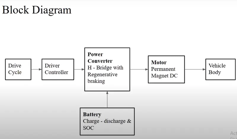
SIMULINK MODEL:-
VEHICAL BODY SUBSYSTEM:-
Tire(Magic Formula):-
The Tire (Magic Formula) block models a tire with longitudinal behavior given by the Magic Formula , an empirical equation based on four fitting coefficients. The block can model tire dynamics under constant or variable pavement conditions.
The longitudinal direction of the tire is the same as its direction of motion as it rolls on pavement. This block is a structural component based on the Tire-Road Interaction (Magic Formula) block.
To increase the fidelity of the tire model, you can specify properties such as tire compliance, inertia, and rolling resistance. However, these properties increase the complexity of the tire model and can slow down simulation. Consider ignoring tire compliance and inertia if simulating the model in real time or if preparing the model for hardware-in-the-loop (HIL) simulation.
Inputs
N - Normal Force:- Physical signal input port associated with the normal force acting on the tire. The normal force is positive if it acts downward on the tire, pressing it against the pavement.
M - Magic Formula CoPhysical signal input port associated with the Magic Formula coefficients. Provide the Magic Formula coefficients as a four-element vector.
Output
S - Slip :- Physical signal output port associated with the relative slip between the tire and road.
Conserving
A _ Axle:-Mechanical rotational port associated with the axle that the tire sits on.
H - Hub:-Mechanical translational port associated with the wheel hub that transmits the thrust generated by the tire to the remainder of the vehicle.
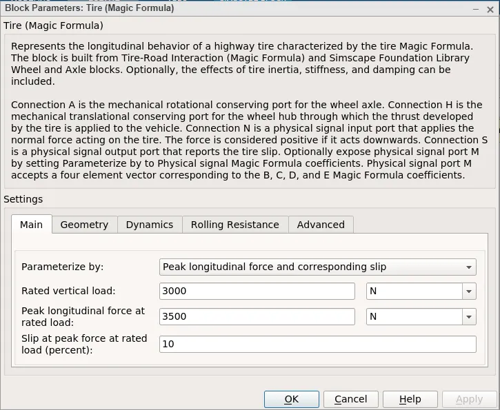
The tires are parameterized by Peak longitudinal force and corresponding slip.
The other block parameters such as - rated vertical load, peak longitudinal force at rated load and slip at peak force at rated load are kept with their default values.
The tire radius is given as 0.3 m.The tire inertia is kept as 1 kg-m^2.
The rolling resistance is given with a constant coefficient of 0.015.
Vehicle Block:-
The Vehicle Body block represents a two-axle vehicle body in longitudinal motion. The vehicle can have the same or a different number of wheels on each axle. For example, two wheels on the front axle and one wheel on the rear axle. The vehicle wheels are assumed identical in size. The vehicle can also have a center of gravity (CG) that is at or below the plane of travel.
The block accounts for body mass, aerodynamic drag, road incline, and weight distribution between axles due to acceleration and road profile. Optionally include pitch and suspension dynamics. The vehicle does not move vertically relative to the ground.
The block has an option to include an externally-defined mass and an externally-defined inertia. The mass, inertia, and center of gravity of the vehicle body can vary over the course of simulation in response to system changes.
Inputs
W - Headwind speed, m/s :- Physical signal input port for headwind speed.
beta - Road incline angle, rad :- Physical signal input port for road incline angle.
CG - Center of gravity, m :- Physical signal input port for the center of gravity, in m, of the externally-defined mass relative to the CG of the vehicle body.
M - Mass, kg :- Physical signal input port for the mass, in kg, of the externally-defined mass.
J - External moment of inertia, kg*m^2 :- Physical signal input port for the moment of inertia, in kg*m^2, of the externally-defined mass.
Outputs
V - Longitudinal velocity, m/s :- Physical signal output port for vehicle longitudinal velocity.
NF - Front axle normal force, N :- Physical signal output port for normal force on the front axle. Wheel forces are considered positive if acting downwards.
NR - Rear axle normal force, N :- Physical signal output port for normal force on the rear axle. Wheel forces are considered positive if acting downwards.
Conserving
H - Horizontal motion :- Conserving port associated with the horizontal motion of the vehicle body. Connect tire traction motion to this port.
Parameters
Vehicle body mass, Centre of gravity distance values and aerodynamic drag variables are modified.Pitch dynamics are kept ON with other variable values as default values
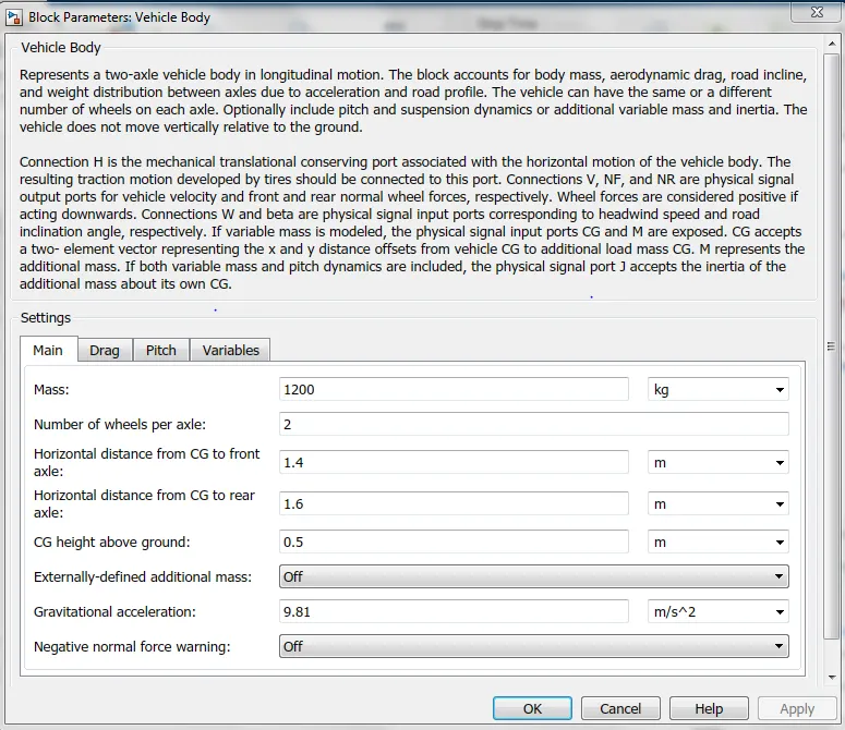
This block basically represents a two-axle vehicle body in longitudinal motion. The block accounts for - body mass, aerodynamic drag, road incline, weight distribution between axles due to accelerationroad profile.
The gross weight is given to be 1200 kg.
Simple Gear:-
The Simple Gear block represents a gearbox that constrains the connected driveline axes of the base gear, B, and the follower gear, F, to corotate with a fixed ratio that you specify. You choose whether the follower axis rotates in the same or opposite direction as the base axis. If they rotate in the same direction, the angular velocity of the follower, ωF, and the angular velocity of the base, ωB, have the same sign. If they rotate in opposite directions, ωF and ωB have opposite signs.
Input
T - External fault trigger :- Physical signal input port for an external fault trigger.
Conserving
B - Base :- Rotational mechanical conserving port associated with the base, or input, shaft.
F - Follower :- Rotational mechanical conserving port associated with the follower, or output, shaft.
H - Heat flow :- Thermal conserving port associated with heat flow. Heat flow affects gear temperature, and therefore, power transmission efficiency.
Parameters
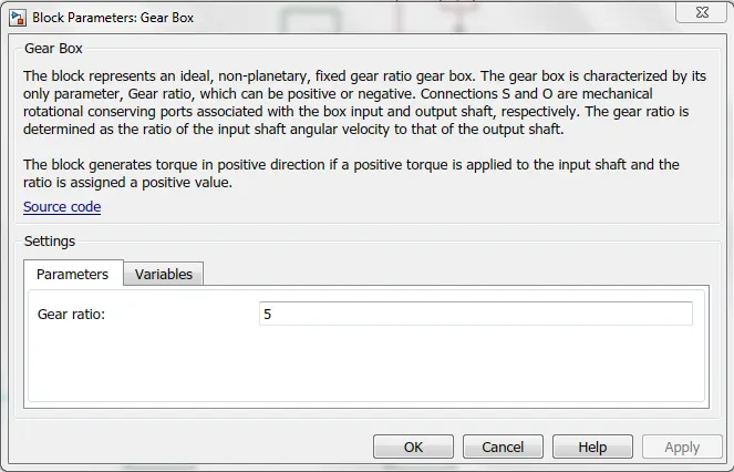
Gear ratio and output direction is modified.Meshing loss is kept constant and gear is having a constant efficiency throughout the simulation.
Viscous losses and faluts are kept at default conditions.
DC MOTOR:-
- Simulink provides an inbuilt bodel block for DC motor which converts electrical input into mechanical rotational output.
- Here, the blue colour corresponds to the electrical side of the motor and the green colour corresponds to the mechanical side.
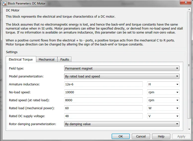
- The motor field type is kept as Permanent magnet and the model parameterization is done by rated load and speed.
- The armature inductance and the mechanical parameters are given their default values.
- The connection R represents the Rotor (rotational output) while the connection C is for the Casing (stationary).
- Thus, the R port is connected to the input of the vehicle subsystem created earlier. The C port is connected to a mechanical rotational reference.
- The + and - terminals of the motor are connected to the motor controller. If these terminals are directly connected to a battery, the required DC motor will run on the rated capacity of the battery.
- This will eventually result into no control over the DC motor and the vehicle will run at top speed throughout the simulation.Thus, a motor controller is very much needed.
- Other parameters are kept constant.
MOTOR CONTROLLER:-
H-Bridge:-
- This block represents an H-bridge motor drive. The block can be driven by the Controlled PWM Voltage block in PWM or Averaged mode.
- In PWM mode, the motor is powered if the PWM port voltage is above the enabled threshold voltage.
- In Averaged mode, the PWM port voltage divided by the PWM signal amplitude parameter defines the ratio of the on-time to the PWM period.
- Connection REF is for the reference input.
- This combined with the PWM connected will form the pulse input for the H-Bridge.
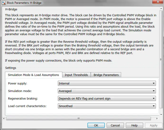
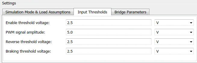
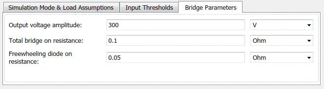
- Here, the REF input is connected to the Electrical Reference (ground).
- Connection REV corresponds to the reverse motion of the motor which essentially means, the backward motion of the vehicle.Here, the backward motion of the vehicle is not accounted for and so, the port is connected to the electrical reference.
- Connection BRK is for the braking of the vehicle.Since, the PWM mode results in a huge amount of simulation time, Averaged mode is selected for this simulation.
- Load current characteristics are considered to be smoothed here.
- Also, the regenerative braking is anabled for the simulation. This means, when the vehicle starts decelerating, corresponding amount of charge will be fed back to the battery.
- Accordingly, the BRK input is connected to a Controlled Voltage Source. This will generate emf corresponding to the intensity of brakes applied and fed the power back to the battery.
Controlled PWM Voltage:-
- The Controlled PWM Voltage Block helps in keeping the Modulated Pulses as per the required pulses.
- So that the operations happens smooth and higher variations are not observed.
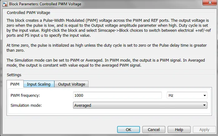
- The Ports are connected as follows,
- ref+ = Reference Positive connected with the Acceleration Commands from the Driver Model.
- ref- = Reference Negative connected with the Deceleration Commands from the Driver Model.
- PWM - PWM connected directly to the H-Block.
- REF - REF connected directly to the H-Block.
- All parameters are set as default.
LONGITUDINAL DRIVER:-
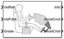
- The Longitudinal Driver block implements a longitudinal speed-tracking controller.
- Based on reference and feedback velocities, the block generates normalized acceleration and braking commands that can vary from 0 through 1.
- You can use the block to model the dynamic response of a driver or to generate the commands necessary to track a longitudinal drive cycle.
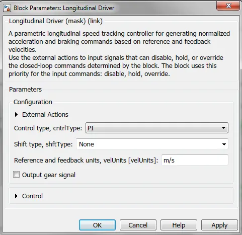
The Driver Model has the Input and Output Ports which are connected to the following,
- Velocity Reference - Drive Cycle
- Velocity Feedback - Distance Calculation
- Grade - Constant 0
- Info - Not Connected
- Acceleration Command - Controlled PWM Source
- Deceleration Command - Brake in H-Bridge to maintain the speed according to the Drive Cycle.
DRIVE CYCLE:-
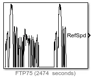
The Drive Cycle Source block generates a standard or user-specified longitudinal drive cycle. The block output is the specified vehicle longitudinal speed, which you can use to:
-
Predict the engine torque and fuel consumption that a vehicle requires to achieve desired speed and acceleration for a given gear shift reference.
-
Produce realistic velocity and shift references for closed loop acceleration and braking commands for vehicle control and plant models.
-
Study, tune, and optimize vehicle control, system performance, and system robustness over multiple drive cycles.
-
Identify the faults within tolerances specified by standardized tests, including:
EPA dynamometer driving schedules and Worldwide Harmonised Light Vehicle Test Procedure (WLTP) laboratory tests.
BATTERY:-
- To model the Battery pak, a simple Battery block is used.
- This is because, if the generic battery block is used instead, the simulation will run for a much longer time.
- Here, the selected option for Battery Charge Capacity is Finite.
- Accordingly, the block models the battery as a series internal resistance plus a charge-dependent voltage source.
- If the chosen option had been Infinite, the voltage source would have been constant.
The battery is connected as the power source to the model so that the power could be generated and the same power is transmitted accordingly to all the operating sources.
The terminals connected are to,
+ - The positive terminal of the operating sources
- - The negative terminal of the operating sources.
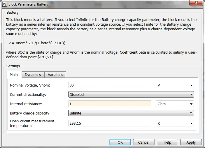
The paramters considered of the battery are :
The battery Nominal Voltage is rated as per 80 Volts.
The internal resistance is as per 1 Ohms and others set as default.
STATE OF CHARGE:-
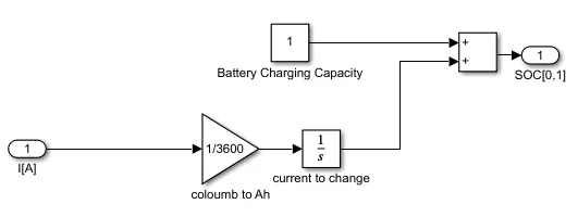
- SOC is calculated by subtracting the charge from the rated capacity of the battery.
- The charge is now converted into percentage value of the charging capacity of the battery.
- Accordingly, the current is integrated w.r.t. time to get the charge in coulumbs.
- Now this coulumb value is modified into Ampere hours.
DISTANCE TRAVELLED:-
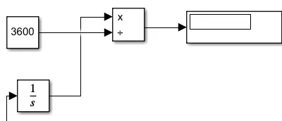
Total distance is calculated as shown from taking the feedback of longitudinal driver.
And connected to display block.
RESULTS:-
Ref Speed vs Actual Speed:-
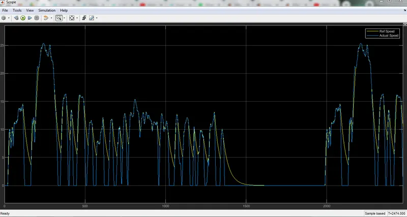
- From above we can be seen from the above picture, the actual velocity of the vehicle slightly differs from the reference drive cycle velocity.
- This is because, the chosen battery capacity and motors are not able to propel the speed upto the required extent.
- If a battery of higher capacity is chosen, the actual velocity will tend to match with the reference velocity.
- Also, it may be noted that in certain regions, despite the drive cycle showing small decelerations, the vehicle actually is accelerating with decreasing magnitudes.
State Of Charge:-
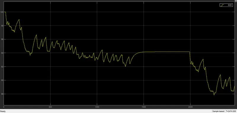
- The State-of-Charge of the battery at the end of simulation run is nearly about 89%.
- This means that the battery is not completely drained at the end and the vehicle can run on the same drive cycle for a few more times before the battery SOC becomes 0.
- Since we had enabled the regenerative braking for the simulation, the battery SOC increases slightly whenever the vehicle undergoes heavy deceleration.
Current:-
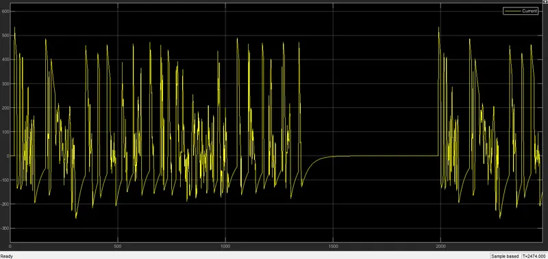
Maximum current is 520A and Minimum current is -250A.
Voltage:-
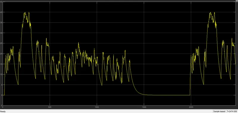
Maximum voltage is 40V.
CONCLUSION:-
Hence, MATLAB model of electric car using a battery and a DC motor is done and results were plotted.
From the above simulation we can conclude that the car has travelled 5.9KM with 80AH battery for the FTP75 Drive Cycle.