FINAL INDEPENDENT PROJECT

AIM:- To study the cause of shock waves and calculate the post-shock condition such as temperature and pressure.

OBJECTIVES:-

• To give a comprehensive report on the formation of shock waves.
• To derive the changes in the properties of a shock wave.
• To analyze the flow after a shock wave, both normal and oblique.

THEORY:-

A shock wave is a thin region in the flow of gas, where the properties like pressure, temperature, flow speed all change very abruptly. The flow of the gas has to be transonic, supersonic, or hypersonic for a shock wave to be formed.

When a jet travels through air, the molecules of air traveling over it are pushed forward. Now, when the speed of the jet is not very high the molecules ahead get the sense of them being pushed forward. But when this happens at a very high speed the molecules are pushed suddenly, creating a thin but very dense layer of air. This layer is called the shock wave. The thickness of a shock wave is of the order of few mean free paths.

There are three types of shock waves:-

1. Normal shock wave
2. Oblique shock wave
3. curved shock wave

For this analysis, we will consider the normal and oblique waves only. The curved shock wave can be analyzed by considering it as a combination of normal and oblique shock waves.

To examine a shock wave we will have to make certain assumptions:-

• Model shock waves as discontinuity.
• Model gas as a continuum.
• Gas is calorically perfect.

RANKINE - HUGONIOT RELATIONS:-

These relations are basically the conservation of mass, energy, and momentum.

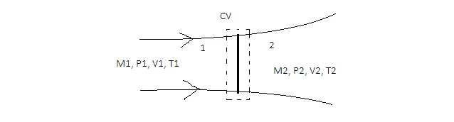
The figure shows a shock wave, with the conditions of properties on either side. For our analysis, we have constructed a rectangular control volume around the shockwave.

Here we can see that the cross-sectional area on both sides of the control volume is the same. So, A1 = A2.

Conservation of mass:-

`rho1* A1* V1 = rho2* A2 * V2`

Since `A1 = A2`

therefore, `rho1* V1 = rho2*V2` ------------------------------------------------------- 1

Conservation of momentum:-

`P1 * A1 - P2 * A2 = rho2* A2 * V2 * V2 - rho1* A1 * V1 * V1`

Since `A1 = A2`

therfore `P1 - P2 = rho2 * V2^2 - rho2 * V1^2` -------------------------------2

Conservation of energy:-

Since the flow is Adiabatic and there is no work done

Therefore, `h1 + 1/2V1^2 = h2 + 1/2V2^2 = h0` ---------------------------------------3

Since the gas is assumed to be perfect

Therefore:- `P = rho*R*T` --------------------------------------------------4

`h = Cp * T` ------------------------------------------------------5

`a^2 = (gammaP)/rho` ---------------------------------------------6

Rearranging these equations:-

Eq. 2:- `(P2)/(P1) - 1 = (rho1*V1^2)/(P1) - (rho2*V2^2)/(P1)`

`(P2)/(P1) - 1 = gamma/gamma(rho1*V1^2)/(P1) (1- (rho2*V2^2)/(rho1*V1^2) )`

`(P2)/(P1) - 1 = gamma(V1^2)/(a1^2)(1-(V2)/(V1))`

By conservation of mass;

`(V2)/(V1) = (rho1)/(rho2)`

Therefore `(P2)/(P1) = 1 + gamma*M1^2(1-(rho1)/(rho2))` --------------------7

Considering the energy equation:-

`Cp *T1 + 1/2*V1^2 = Cp*T2 + 1/2*V2^2`

`(T2)/(T1) = 1+(1/2*V1^2)/(Cp*T1) - (1/2*V2^2)/(Cp*T2)`

`= 1 + (1/2*V1^2)/(Cp*T1)*(1- ((V2)/(V1))^2)`

Since `a1^2 = gamma*R*T`

and `Cp = R*(gamma)/(gamma-1)`

Therefore `(T2)/(T1) = 1 + (gamma-1)/2*M1^2(1-((rho1)/(rho2))^2)` ---------8

From the ideal gas equation, `(T2)/(T1) = (P2*rho1)/(P1*rho2)` --------------------------------------9

using eq. 7:-

`(T2)/(T1) = (1 + gamma*M1^2(1-(rho1)/(rho2)))*(rho1)/(rho2)` -------10

from equations 8 and 10, we get:-

`1 + (gamma-1)/2*M1^2(1-((rho1)/(rho2))^2)``= (1 + gamma*M1^2(1-(rho1)/(rho2)))*(rho1)/(rho2)`

which is a quadritic equation of `(rho1)/(rho2)`.

on solving this quadritic equation, we get two solutions:-

• `rho1 = rho2`
• `(rho2)/(rho1) = ((gamma +1)*M1^2)/(2 + (gamma-1)*M1^2)`

On putting these values in equations 8 and 9, we get:-

• `(P2)/(P1)=``(2*gamma*(M1^2)-gamma+1)/(gamma+1)`
• `(T2)/(T1) = ((2*gamma*(M1^2)-gamma+1)*((gamma-1)*(M1^2)+2))/((gamma+1)^2*(M1^2))`

We can also calculate the value of post-shock Mach number:-

`M2=(V2)/(a2) = (V2)/(V1)*(V1)/(a1)*(a1)/(a2)`

therefore, `M2 = (rho1)/(rho2)*M1*root2((T1)/(T2))`

Putting the values of the ratios, we get:-

`M2 = root2((1+(gamma-1)/2*M1^2)/(gamma*M1^2-(gamma-1)/2)`

So, we have expressed several ratios and post_shock Mach number in terms of pre-shock Mach number and gamma (ratio of specific heats).

Here is the code for calculating the variation of different ratios with respect to the initial Mach number:-

The code has been divided into two parts. The first is the function that contains the formulae of the ratios, and the second one calculates and plots the ratios with respect to the Mach number range.

First part

% 1 represents pre-shock condition
% 2 represents post-shock conditions

function f = rankine_hugoniot(M1,y)

% density ratio rho2/rho1

density_ratio  =  ((y+1)*(M1^2))/(2+(y-1)*(M1^2));

% pressure ratio P2/P1

pressure_ratio = (2*y*(M1^2)-y+1)/(y+1);

% temperature ratio T2/T1

temperature_ratio = ((2*y*(M1^2)-y+1)*((y-1)*(M1^2)+2))/((y+1)^2*(M1^2));

f=[density_ratio ; pressure_ratio ; temperature_ratio];
end

Second part

% determining the post-shock condition of properties 
clear all 
close all
clc

% 1 represents pre-shock condition
% 2 represents post-shock conditions


% pre-shock conditions
M1 = linspace(1,10,10);              % initial mach numbers
y  = 1.4;                            % ratio of specific heats, assumed constant

for i = 1: length(M1)
output(i,:) = rankine_hugoniot(M1(i),y);
end

figure(1)
plot(M1,output(:,1),'linewidth',1,'color','b')
xlabel('initial Mach number M1')
ylabel('density ratio    rho2/rho1')
axis([1 10 0 6])
title('density ratio variation')
grid on

figure(2)
plot(M1,output(:,2),'linewidth',1,'color','r')
xlabel('initial Mach number M1')
ylabel('pressure ratio    P2/P1')
title('pressure ratio variation')
grid on

figure(3)
plot(M1,output(:,3),'linewidth',1,'color','g')
xlabel('initial Mach number M1')
ylabel('temperature ratio  T2/T1')
title('temperature ratio variation')
grid on

figure(4)
plot(M1,output(:,4),'linewidth',1)
xlabel('initial Mach number M1')
ylabel('final Mach number M2')
title('Post shock Mach number variation')
axis([1 11 0 1.5])
grid on

Here are the plots for the variations:-

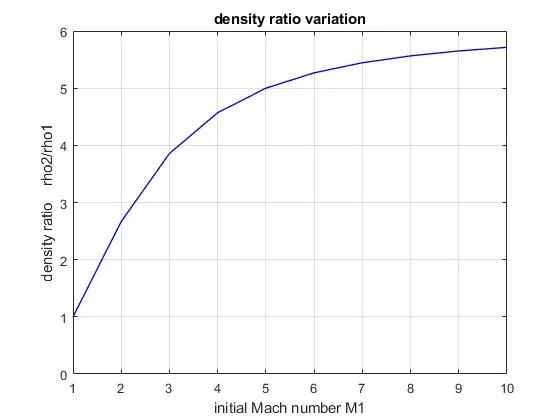
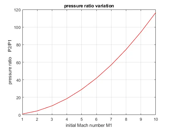
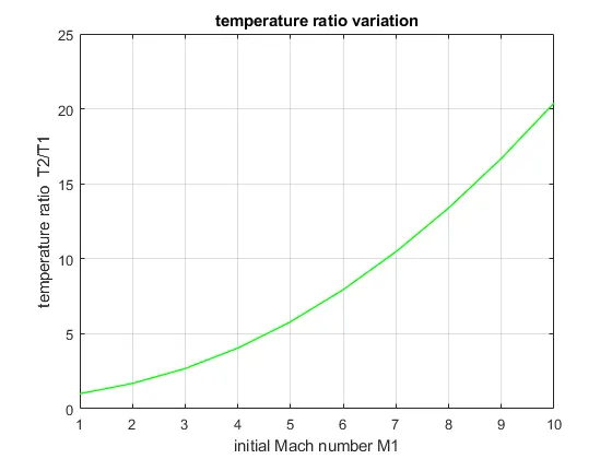
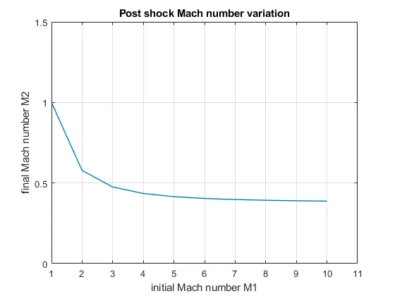
From the last graph, we see that the flow on the other side of the shockwave is subsonic:-

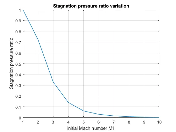
Loss associated with Normal shock wave:-

P01 --> Pre-shock stagnation pressure

P02 --> Post-shock stagnation pressure

`P01 = P1*(1+(gamma-1)/2*M1^2)^(gamma/(gamma-1))`

`P02 = P2*(1+(gamma-1)/2*M2^2)^(gamma/(gamma-1))`

Putting the values of `(P2)/(P1)` and M2:-

`(P02)/(P01)=(((gamma+1)*M1^2)/(2+(gamma-1)*M1^2))^(gamma/(gamma-1))*((gamma+1)/(2*gamma*M1^2-gamma+1))^(1/(gamma-1))`

Here is the graph depicting the loss in the stagnation pressure with an increase in Mach number:-

Oblique shock wave analysis:-

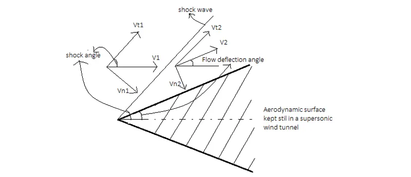
Flow deflection angle -->`theta`

shock angle ------------>`beta`

The subscript 't' and 'n' represent the tangential and normal component respectively.

V1 is the initial velocity of the oncoming wind. V2 is the velocity after the shock. This deflection is in the direction of the plane.

Basically, the oblique shock wave is just the normal shock wave inclined at some angle.

Tangential direction analysis:-

Applying momentum conservation,

Since there is no force in the tangential direction.

`sumft = int(rho*V*dA)*Vt`

`0=m*(Vt2-Vt1)`

`Vt2 = Vt1`

So we see, that there is no change in the tangential component of velocity across an oblique shock wave.

Normal direction analysis:-

For the normal component of velocity, the oblique shock wave behaves like a normal shock wave. Therefore, all the relations of the normal shock wave can be used here.

`P1-P2=rho2*Vn2^2 - rho1*Vn1^2`

Continuity equation, `rho1*Vn1 = rho2 *Vn2`

Energy equation, `h1+1/2*Vn1^2=h2+1/2*Vn2^2`

Therefore all the normal shock wave relations can be used here, just by replacing the Mach numbers with their normal components.

`Mn1=M1*sinbeta`

`Mn2=M2*sin(beta-theta)`

Therefore,

• `(rho2)/(rho1) = ((gamma +1)*Mn1^2)/(2 + (gamma-1)*Mn1^2)`

• `(P2)/(P1)=``(2*gamma*(Mn1^2)-gamma+1)/(gamma+1)`

• `(T2)/(T1) = ((2*gamma*(Mn1^2)-gamma+1)*((gamma-1)*(Mn1^2)+2))/((gamma+1)^2*(Mn1^2))`

Since, `(Vn1)/(Vn2)=(Vt1*tanbeta)/(Vt2*tan(beta-theta)`

and `Vt1=Vt2`

Therefore, `(Vn1)/(Vn2) = tanbeta/tan(beta-theta)`

By continuity equation,

`tanbeta/tan(beta-theta)``=((gamma +1)*Mn1^2)/(2 + (gamma-1)*Mn1^2)`

Here is the code to solve this equation for `theta`:-

clear all
close all
clc

M1 = linspace(1,8,8);      % range of pre-shock Mach number
y = 1.4;
B = linspace(1,100,100);     % shock angle beta

% using nested for loop to plot the graph for different values of Mach number M1

for j = 1:length(M1)
    for i = 1:length(B)
      theta(i) = B(i)- atand(((2+(y-1)*M1(j)^2*sind(B(i))^2)/((y+1)*M1(j)^2*sind(B(i))^2))*(tand(B(i))));
    end
    plot(theta,B)
    hold on
end
axis([0 60 0 100])
grid on
gtext('M1=1')
gtext('M1=2')
gtext('M1=3')
gtext('M1=4')
gtext('M1=infinite')

Here is the graph showing the variation of shock angle `beta` with changing angle of deflection `theta`:-

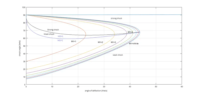
Therefore, we can conclude that for any given M1 and `theta`, we have two solutions:-

• Weak shock solution (Low `beta`)
• Strong shock solution (High `beta`)

We also see, that for a given M1 there is a maximum angle of deflection for which a shock is possible. If we join these points we get a curve, which has a strong shock solution above it and a weak shock solution below it.

Usually, M2>1 downstream for weak shock, i.e the flow remains supersonic downstream for a weak shock, and M2<1 always, for a strong shock.