Exhaust Port Challenge

Abstract:

In the present study, A conjugate heat transfer analysis is conducted on an exhaust pipe manifold and to study the heat transfer across the manifold. In this study the average heat transfer coefficient along the internal surface was obtained based on the diameter of the exhaust pipe. The temperature and the velocity contours were drawn.

Introduction:

Exhaust manifold is an important part of any propulsion systems. Exhaust manifolds are generally made of simple cast iron or stainless steel. It collects hot exhaust gases from the engine tat are produced after combustion and release them to the atmosphere(the flow is the result of pressure difference across the manifold, higher pressure at the engine exit and at the exit of the manifold the pressure is atmospheric. Since at the exit of the engine the exhaust gases are at higher temperature and these temperatures will get transferred to the exhaust manifold, it is required to conduct the heat transfer analysis so that the temperature variations within the manifold which might add up to the physical stresses in the form of thermal stresses can be identified and according to that design can be optimized.

Conjugate heat transfer:

In a System where heat transfer is due to more than one mode of heat transfer can be called as conjugate heat transfer problems. CHT analysis helps in obtaining the heat transfer values accurately by solving relevant conduction convection and radiation equations simultaneously. CHT Has an advantage over Solving the finite element thermal analysis in which empirical formulas will be used in getting the results whereas in CHT approach the local variations in heat transfer coefficients over the surfaces were directly calculated within the model.

Many thermal engineering problems are generally comes under the category of conjugate heat transfer.

For example, exhaust manifold where the heat transfer is due to conduction and convection similarly in heat exchangers the same phenomenon can be observed.

Modelling approach:

The present model basically is a body that exists at the end of the engine connected to the engine exhaust at one end and the other to the muffler or exposed to atmosphere. It means hot exhaust enters at one end at little higher pressure than ambient in order to compensate the pressure losses along the manifold. Within the model we have two different volumes one is solid volume which is made of aluminium and the control volume in which exhaust flows. The outer surface of the solid volume is exposed to convection boundary conditions. The meshing was done in such a way that there is a perfect contact between fluid and solid volumes using share topology share prepare. Since the flow to be turbulent the models selected are to be turbulent. Two equations models are most used, k e and k, w models.

Since the fluid coming from an engine where turbulence is generally induced for better mixing this adds to the turbulence that is inherent to that of the flow. This requires the turbulence intensity to be increased. The cell zone conditions should be checked for proper matching with those of required materials. Within the reference values the reference length should be changed to that of the diameter of the flow. Different algorithms are available for solving the equations like COUPLED, SIMPLE, SIMPLEC etc.. after selecting the models convergence criteria can be changed in residuals. By plotting residuals against iterations one will be able to identify whether the solution is getting converged are not. In the present model hybrid initialization is done which uses some random values and checks whether the solution is getting converging or diverging, according to that we may need to make necessary changes to the mesh.

Geometry:

The geometry contains four inlets connected to common manifold and a single outlet. All the inlets are circular and are of same diameter.

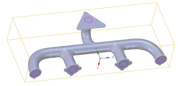
Those pink circles represent the shared topology between solid and fluid volumes.

Meshing:

on the outer shell body sizing was done and at the interface between fluid and solid volume inflation is applied and for the element closer to the wall the y+ value was ensured to be less than one in order to consider laminar sublayer. The y+ value was calculated from solvers available in internet

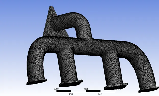
the meshed model

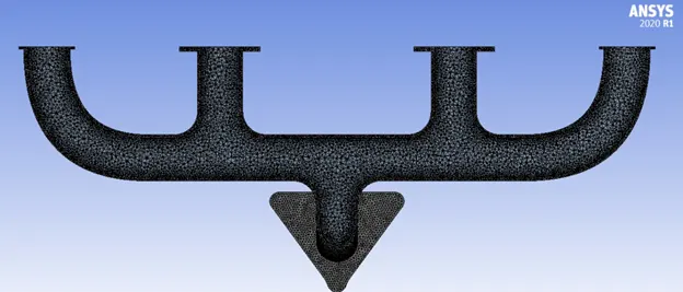
the section view of the model

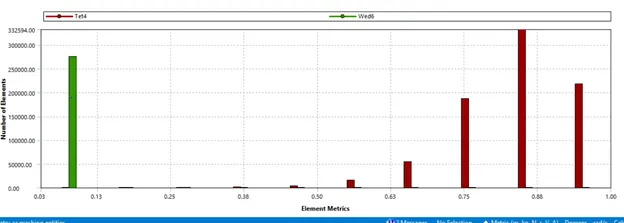
Element quality

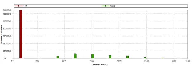
Aspect ratio

Grid independence test:

In the present study two different grids were used for the simulation and the bulk mean temperature at the outlet was used as the parameter for testing the grid independency and are listed below:

serial	Grid size	Temperature(K)	% change
1	495000	677.5219	--
2	1087000	677.37194	0.02214

There is no much variation in the value of temperature by changing the grid size. So it is fine to use coarse grid for the present model.

Boundary conditions:

The fluid in the present model is considered as air and the material of the manifold is considered as aluminium. At the inlets of the exhaust manifold, the velocity of air is taken as 5 m/sec with an turbulence intensity as 10% and the temperature of the fluid to be 700 k. at the outlet gauge pressure was made zero. On the outer surface of the manifold convection boundary conditions are applied with heat transfer coefficients of 20 w/m2k. remaining portions of the wall are adiabatic.

Solution methodology:

With the energy equation on and the turbulent model selected the system need to solve 7 equations all together, which include energy, momentum, continuity and two equations of turbulence model(in this case I have used SST kw model and hence equations of k and w). for solving conservation equations COUPLED equation solver is used.

Governing equations:

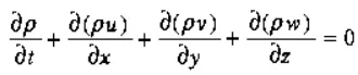
The fluid domain considered to be incompressible and governing equations satisfying the fluid domain are given below:

Continuity equation:

X-momentum equation:

Y-momentum equation:

Z-momentum equation:

For non-dimensionalization considering following parameters,

By Non-dimensioning the governing equations becomes:

Continuity equation:

X-momentum equation:

Y-momentum equation:

Z-momentum equation:

Where, Re = Reynolds number (𝜌𝑢𝑑/𝜇)

Results:

the temperature contour of the domain with the streamlines in it

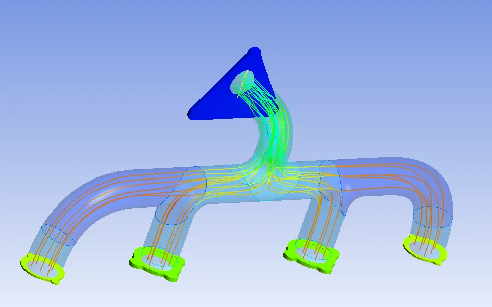
one can observe that in the outlet art of the manifold the streamlines are closer or otherwise say are denser, this is due to the fact that mass is always conserved. since it has four inlets and only one output, the mass flow rate through the outlet is four times that of the inle.

the temperature contour of the Z plane:

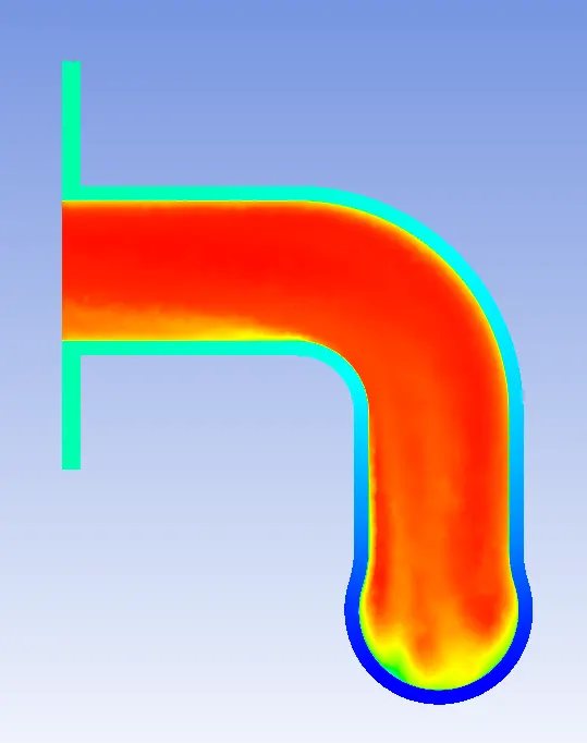
the velocity contour of the z plane

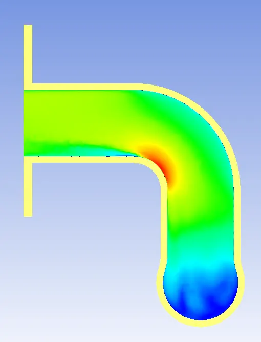
wall heat tranfer coefficient:

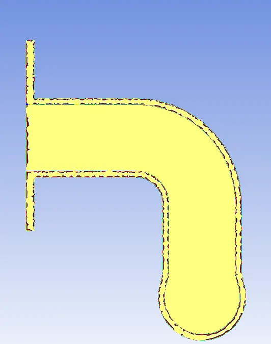
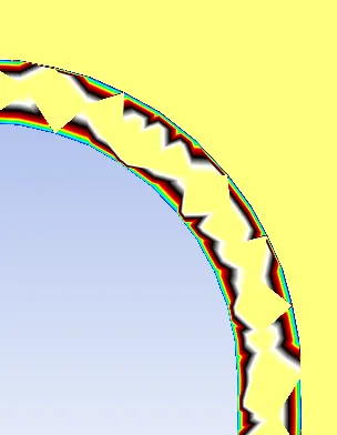
average heat transfer coefficient on the inner surface of the manifold is 25.4016 W/m2k

the results obtained from cfd solvers generally required to be validated for tis the results need to be compared with that of the experimental values or those results from the journals. for this people genrally do simple case simulations with the similar setup and generally compare with the experiment and if the results are satisfactory then one can continue with the complex simmulation.

Conclusion:

the velocity and temperature contourrs were drawn.

the contourof heat transfer coefficient and also the average heat transfer coefficient value is obtained.