Conjugate heat Transfer Simulation of Exhaust Port using Ansys Fluent

Exhaust Port Simulation

Conjugate Heat Transfer and its Significance:

The term conjugate heat transfer (CHT) is used to describe processes which involve variations of temperature within solids and fluids, due to thermal interaction between the solids and fluids. The exchange of thermal energy between the two physical bodies is called the study of Heat Transfer, the rate of transferred heat is directly proportional to the temperature difference between the bodies. A typical example is the heating or cooling of a solid object by the flow of air in which it is immersed and some other example includes conduction through solids, free and forced convection in the gases/fluids and thermal radiation.

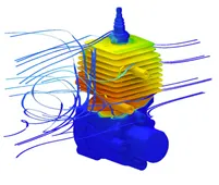
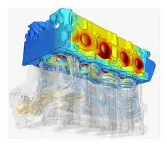
Conjugate heat transfer corresponds with the combination of heat transfer in solids and heat transfer in fluids. In solids, conduction often dominates whereas in fluids, convection usually dominates. Efficiently combining heat transfer in fluids and solids is the key to designing effective coolers, heaters, or heat exchangers. Forced convection is the most common way to achieve high heat transfer rate. In some applications, the performances are further improved by combining convection with phase change (for example liquid water to vapor phase change).

Heat transfer in solids and heat transfer in fluids are combined in the majority of applications. This is because fluids flow around solids or between solid walls, and because solids are usually immersed in a fluid.

The fluid flow and heat transfer problems can be tightly coupled through the convection term in the energy equation and when physical properties are temperature dependent. While analytical solutions exist for some simple problems, we must rely on computational methods to solve most industrially relevant applications.

CHT can be performed to improve cooling performance of the water jacket and increase engine life. Advancements in cooling for applications such as gas turbines components require improved understanding of the complex heat transfer mechanisms and the interactions between those mechanisms. Critical cooling applications often rely on multiple thermal protection techniques, including internal cooling, external film cooling, etc. which are efficiently used by CHT analysis to cool components and limit the use of coolant. For Motor and Battery CHT Analysis to get optimized design for High voltage systems. Conjugate Heat Transfer analysis provides the temperature distribution in solid and coolant of the engine and clear insight on velocity distribution and mechanism of heat transfer of coolant. Results of CHT analysis become input to structural simulations as thermal loads.

CHT Analysis for various type of engines like Bikes, Passenger Cars, Racing cars, Commercial Vehicles, Marine, Agricultural equipment and Earth-moving equipment etc.

Modes of heat transfer

• Conduction: diffusion of heat due to temperature gradients. A measure of the amount of conduction for a given gradient is the heat conductivity.
• Convection: when heat is carried away by moving fluid. The flow can either be caused by external influences, forced convection; or by buoyancy forces, natural convection. Convective heat transfer is tightly coupled to the fluid flow solution.
• Radiation: transfer of energy by electromagnetic waves between surfaces with different temperatures, separated by a medium that is at least partially transparent to the (infrared) radiation. Radiation is especially important at high temperatures, e.g. during combustion processes, but can also have a measurable effect at room temperatures.

Heat Transfer Coefficient and its Prediction

Heat transfer coefficient, often denoted by hx or h¯h¯ and measured in Wattm2⋅KWattm2⋅K, is a quantitative characteristic of convective heat transfer, typically between a surface and a medium, which relates heat flux qs,x˙′′qs,x˙″with the temperature difference between the surface and the medium. For steady state heat transfer i.e. when ∂T∂t=0∂T∂t=0,

qs,x˙′′=hx⋅(Ts−T∞)qs,x˙″=hx⋅(Ts−T∞)

Here hx is the localized heat transfer coefficient at xx, TsTs is the surface temperature of the object from which heat is being transferred, and T∞T∞ is the ambient temperature.

The overall heat transfer coefficient can be calculated as follows:

h¯=∫Ahx⋅dAh¯=∫Ahx⋅dA

Thus, heat transfer rate q˙=h¯⋅A⋅(Ts−T∞)q˙=h¯⋅A⋅(Ts−T∞).

There is one more equation which relates heat flux with the temperature gradient:

q˙′′=−kf(∂T∂y)q˙″=−kf(∂T∂y)

Here, kf is the thermal conductivity of the medium (unit: Wattm⋅K), which measures its ability to conduct heat.

Combining the equations and multiplying by length of the surface, we get a dimensionless number called Nusselt Number NuNu which is the ratio of heat transferred through convection to the heat transferred through conduction. In simple terms, it tells us how much the heat transfer is enhanced due to fluid motion. Hence HTC is depend on Nussselt number.

`Nu¯=(h¯⋅L)/(kf)`

A lot of calculations related to heat transfer coefficient can be done by using certain statistically established correlations involving the Nusselt number and other dimensionless numbers like Reynolds number and Prandtl number.

Factors affecting HTC:

1. Velocity of the fluid.
2. Density of the fluid.
3. Viscosity of the fluid.
4. conductivity of the fluid.
5. Characteristic length of the heat transfer area.
6. Heat capacity of the fluid.
7. Temperature difference between the hot and cold body.
8. Mean film temperature of the fluid.

Steps in Simulation:

Open Ansys Workbench. Drag and drop Fluid Flow (Fluent) onto Project Schematic.

Here, we will see Steps we need to follow to solve a particular engineering system from a CFD standpoint.

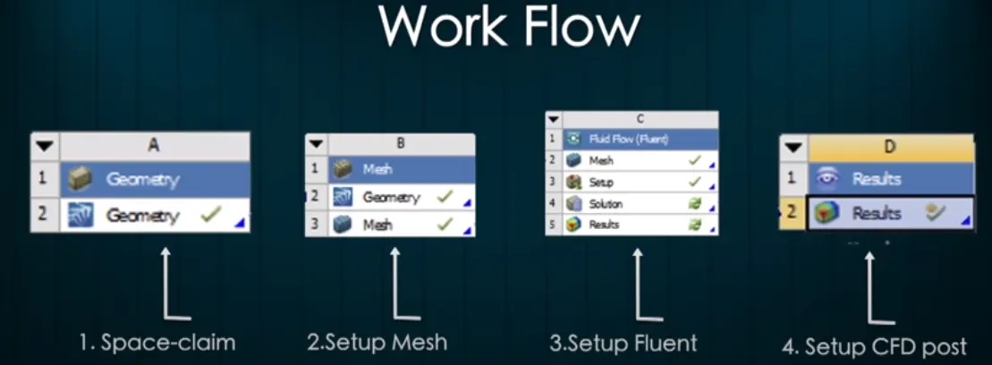
1. Geometry: Spaceclaim, where we import the geometry.
2. Mesh: Ansys Mesh, where Boundary naming, element sizing and mesh generation with required grid size will be done.
3. Setup: Ansys Fluent, where actual case setup will be done.
4. Solution: Ansys Fluent, where runtime results visualization done.
5. Results: CFD-Post, where Post Processing of Results will be done.

CAD Cleanup:

Import Exhaust Port geometry into Spaceclaim, Spaceclaim is CAD cleanup software that can be used to prepare CAD models for simulation setup. It could be for CFD or FEA.

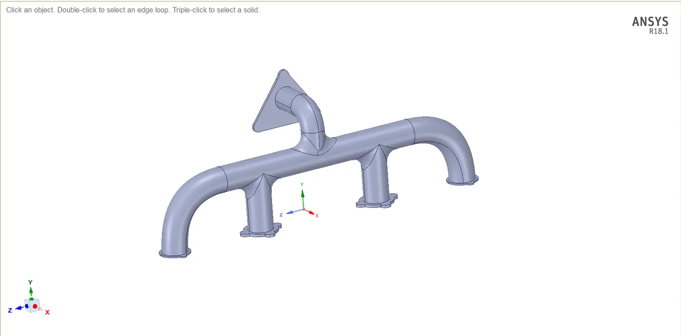
As we can see above figure is the Solid model. We have a solid model of an Exhaust Port inline 4-cylinder engine and then we are going to modeling both the fluid flow through it and also the Heat Transfer coefficient.

• Extract the Fluid volume- Go to Prepare ->Volume extract ->select edges ->ok. Now we have two-volume. i.e, Fluid volume, and Solid volume.
• Enable Share topology to share the entire interface information between Solid and Fluid
• and also to avoid any gaps between these two Solid and Fluid volumes(i.e to have a Conformal Mesh), enable Share ->go to Workbench->select FFF-> click Share/Shareprep

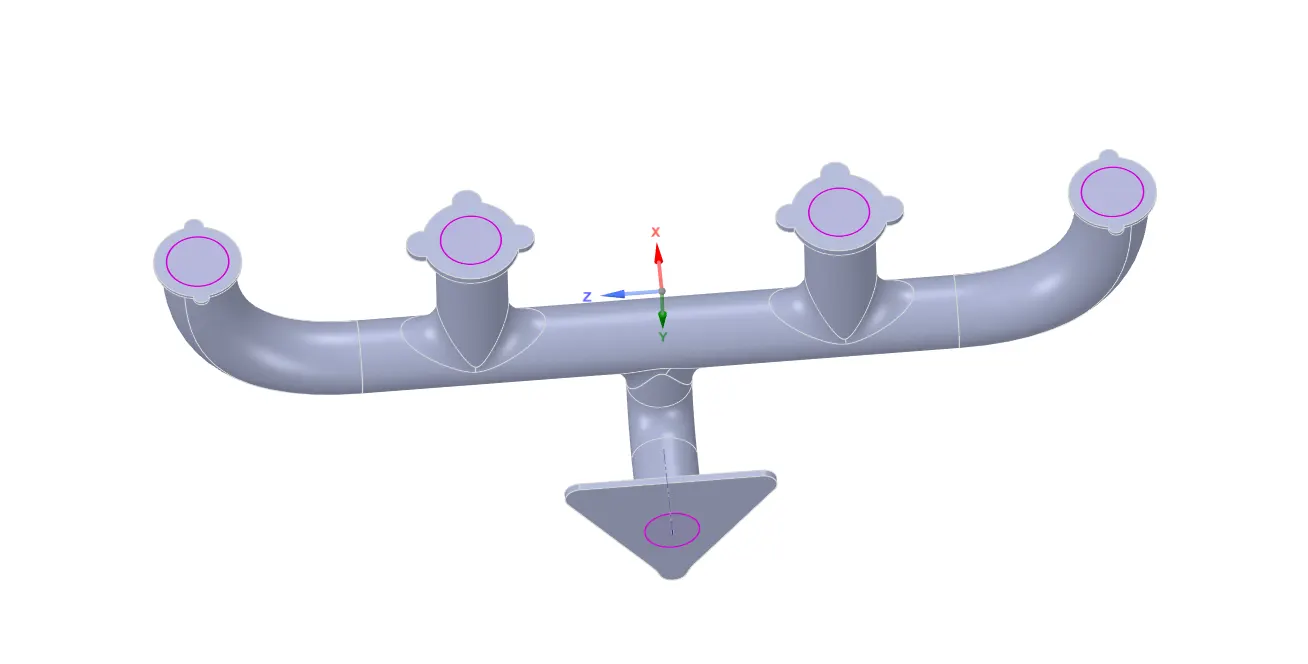
These pink edges show that, the geometry os Conformal.

Mesh Generation

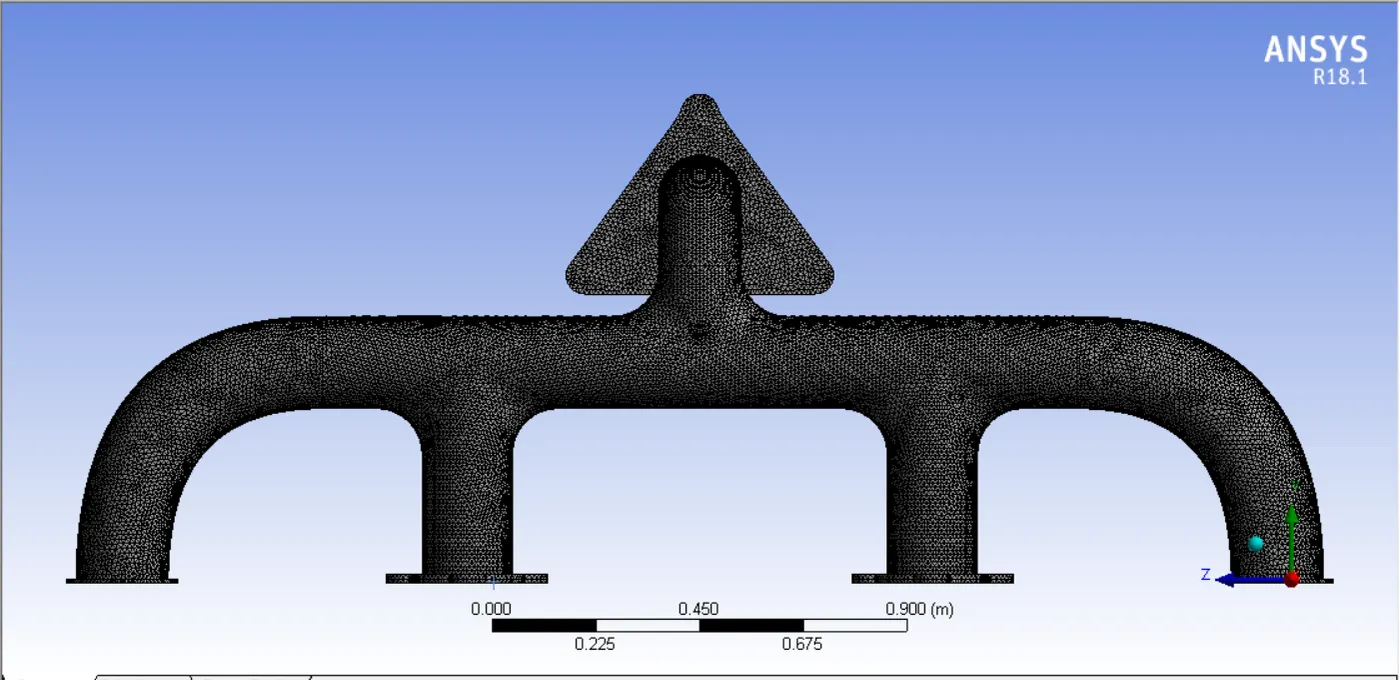
Baseline Mesh:

• Generate Mesh

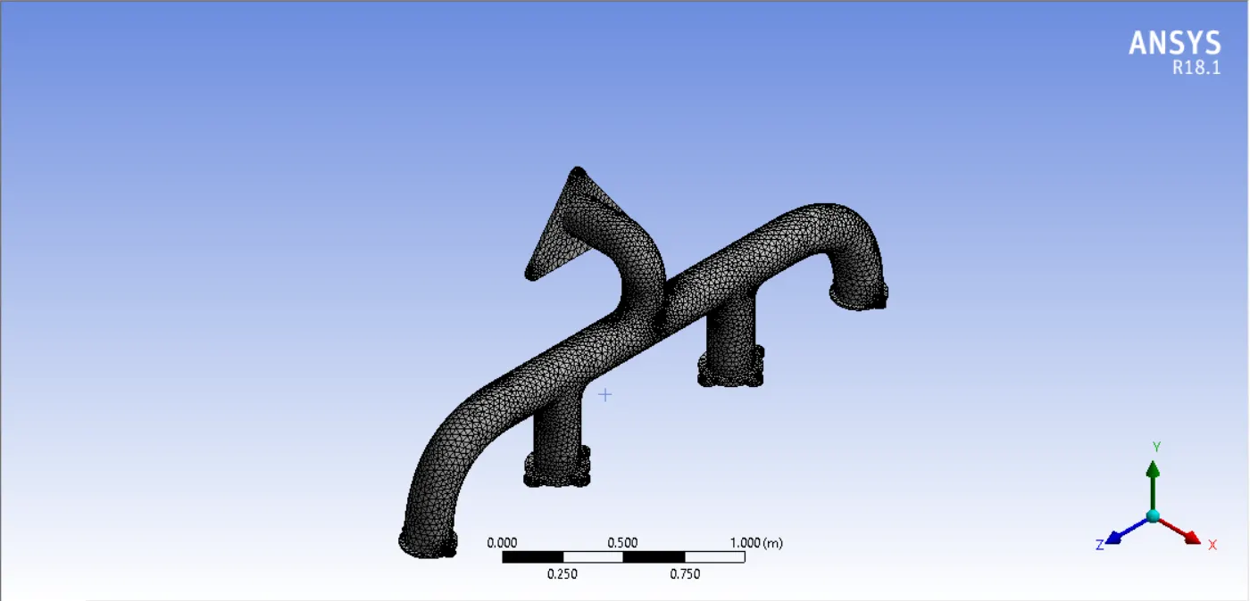
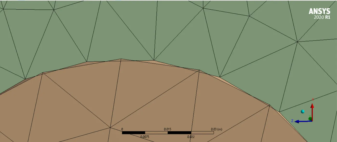
Now we can see that, the above mesh has not a common interface between solid and fluid volume, hence it is undesirable. For this we to enable share topology and Shareprep option enabled, so to get a Conformal mesh

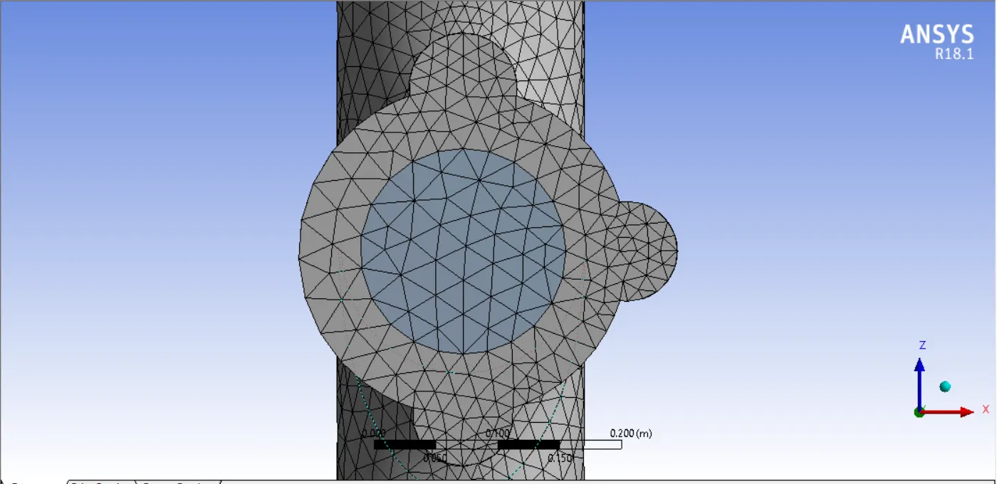
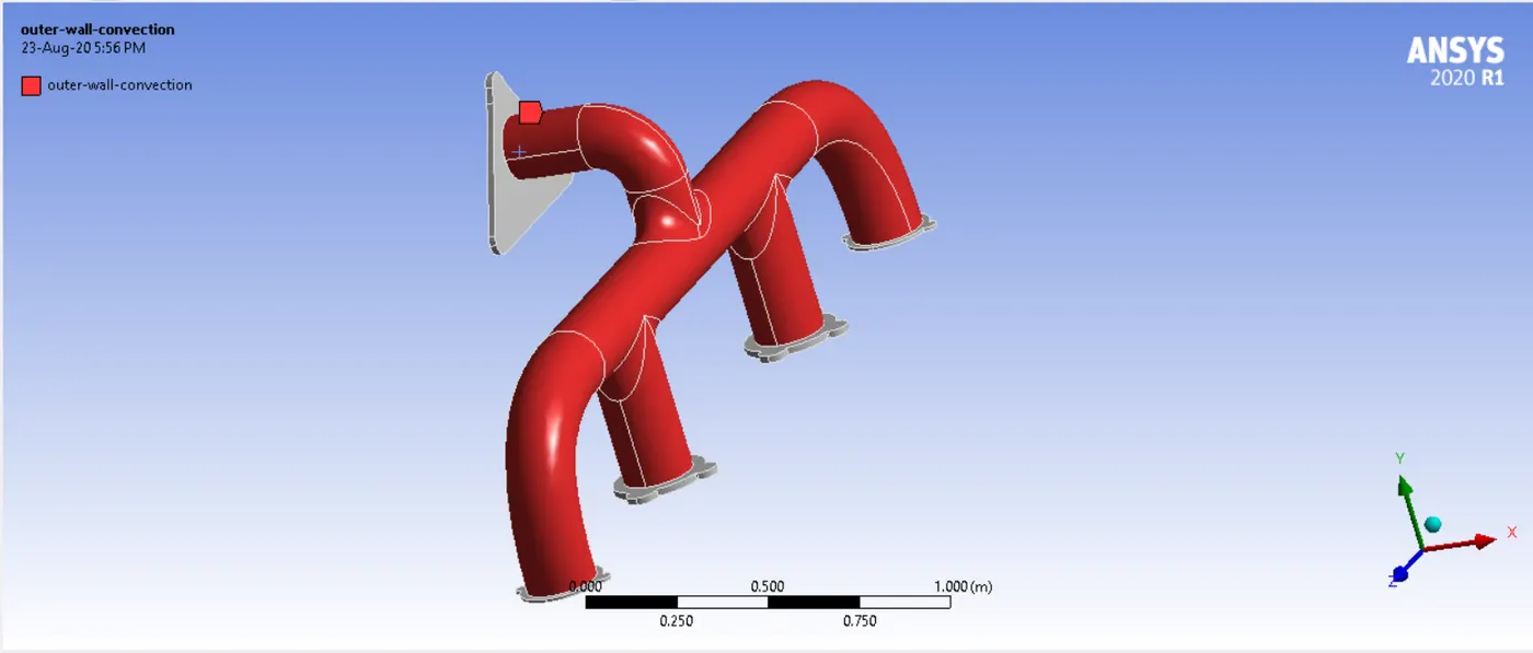
• Name Selection: Inlet(4-ports through which the hot gases will enter), outlet and Outer-wall-convection(Outer solid surface).
• Outer-wall-convection

Refined Mesh:

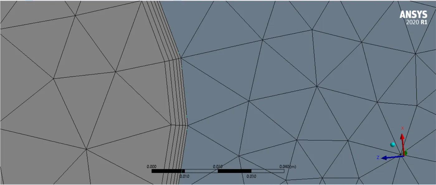
Wrong inflations

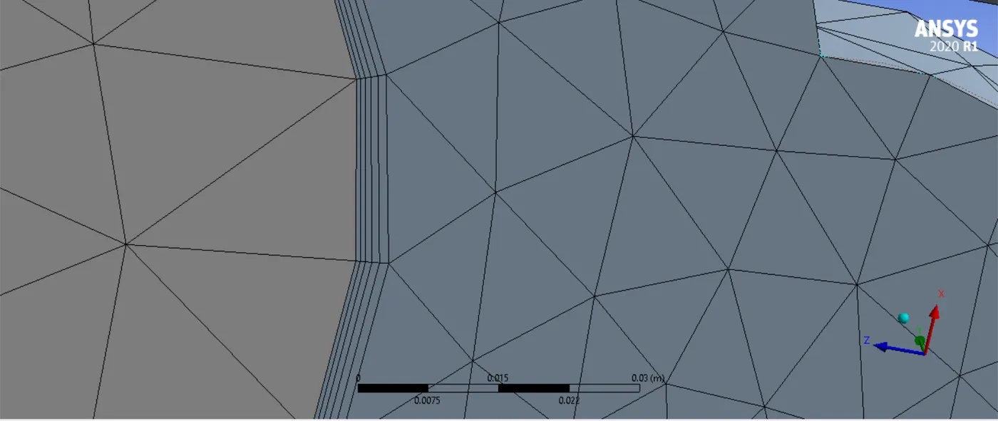
Correct Inflation

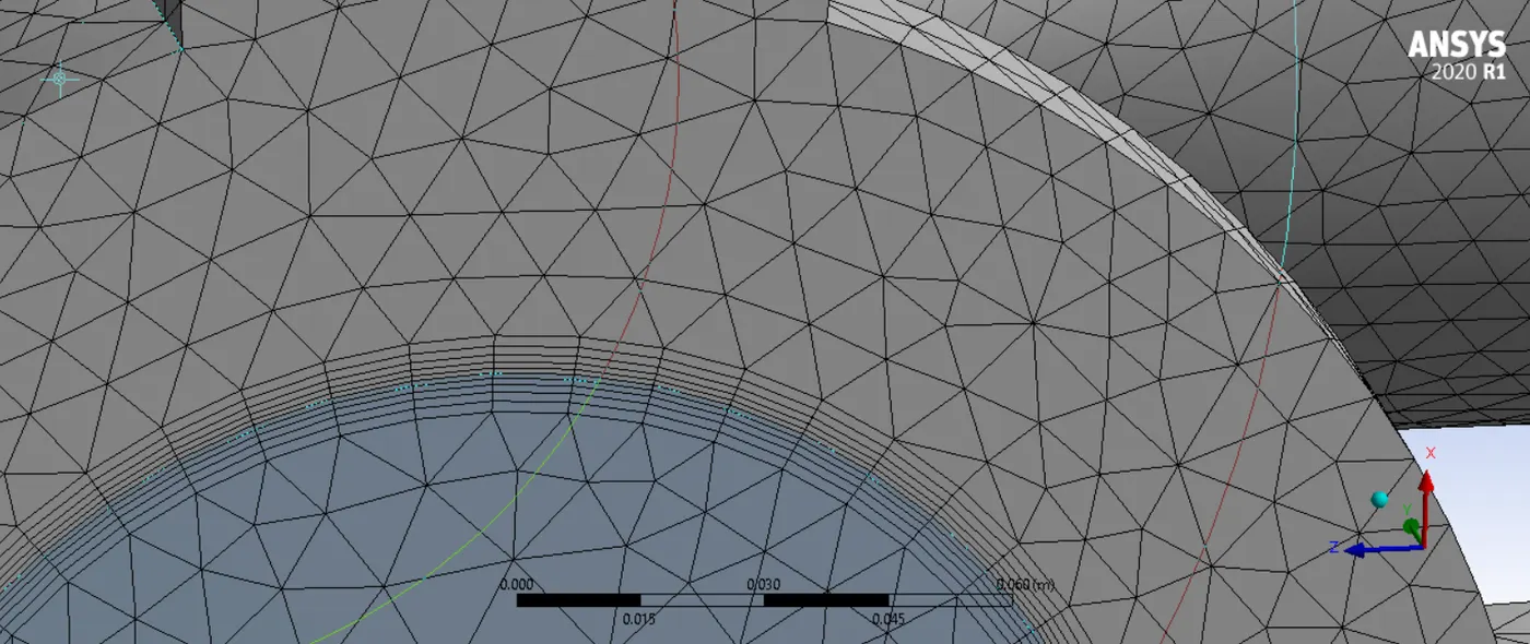
The inflation layers must be created on both the sides of Solid and fluid volume

For this select below fluid volume with excepting Inlets and Outlet as shown below

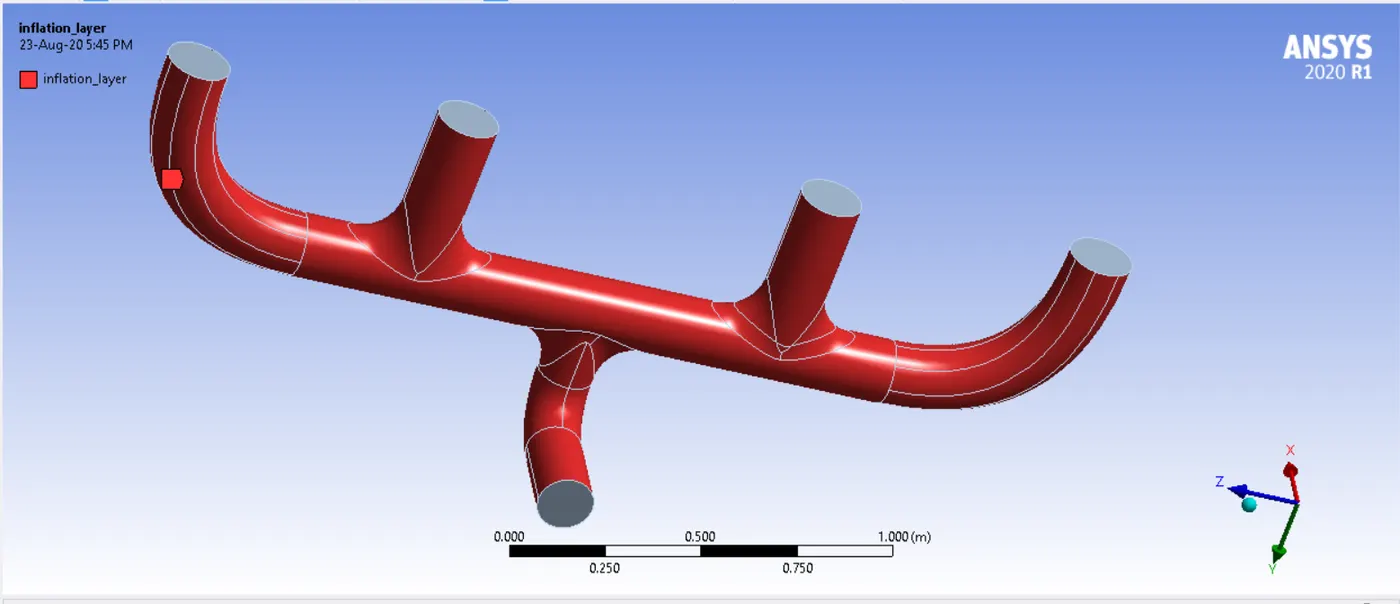
Add Inflation Layer of total thickness of 3mm from calculating the y-plus=100 using y+ online calculator.

Assign Element size of solid component 10mm.

Fluent Setup:

Setting up physics: Select k-epsilon Standard terbulent model

Solver: Pressure-based.

Assign Time as Steady-State Solver.

Material Selection:

For Fluid- Air

For solid- aluminium.

Properties of Material:

Density of Air = 1.225 kg/m^3

Density of Solid = 2719 kg/m^3

Setting Boundary Condition:

For Inlet:

Velocity t= 5m/s

Temperature = 700kelvin

Outlet:

Pressure= 0 Pascal. (Ambient Pressure)

Outer-wall-convection:

Heat transfer coefficient=20w/((m^2)*k)

Assigning different Flow quantities:

• Create Temperature contour
• Hybrid Initialize and run the Simulation for 150 iterations.

CFD Result:

• Create Velocity and Pressure contour in entire exhaust port and also at throat.
• Check heat Transfer Coefficient at the wall.

Plots:

Baseline Mesh:

Temperature streamline:

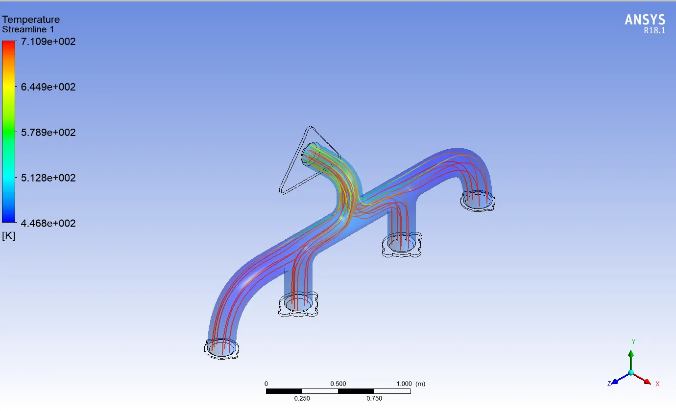
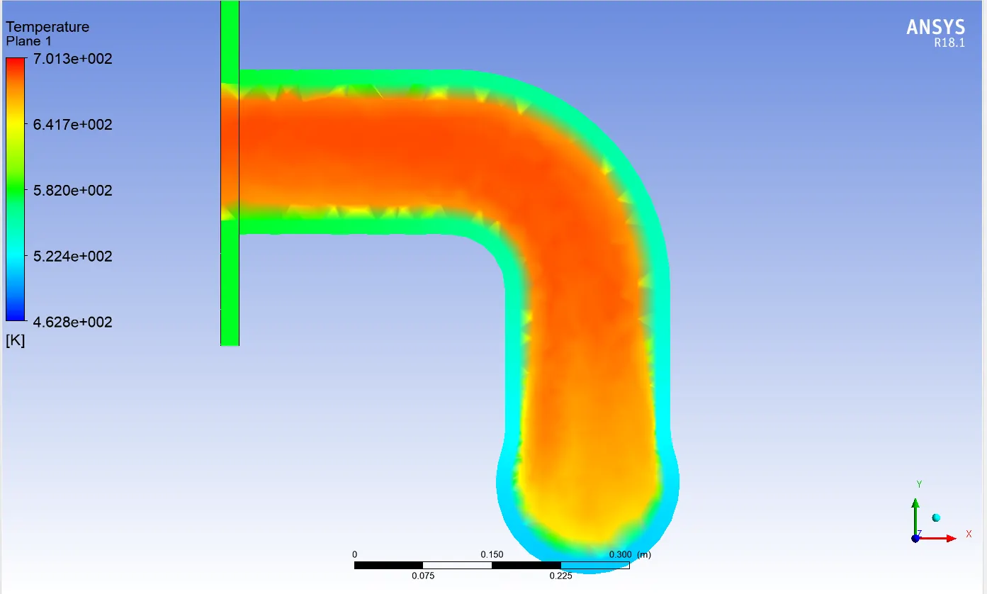
Temperature lowers at the throat due to high Heat Transfer rate.

Velocity Streamline:

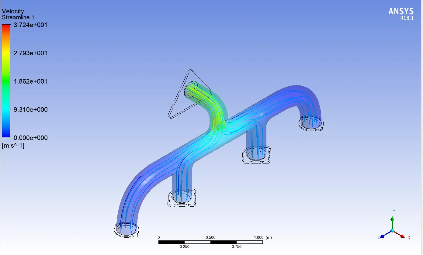
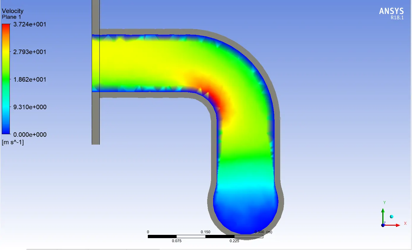
The Velocity at the throat increases due to incoming gases from all the four inlet.

Temperature at the Exit port throat:

Velocity at the Throat:

Heat Transfer coefficient of inner solid Wall:

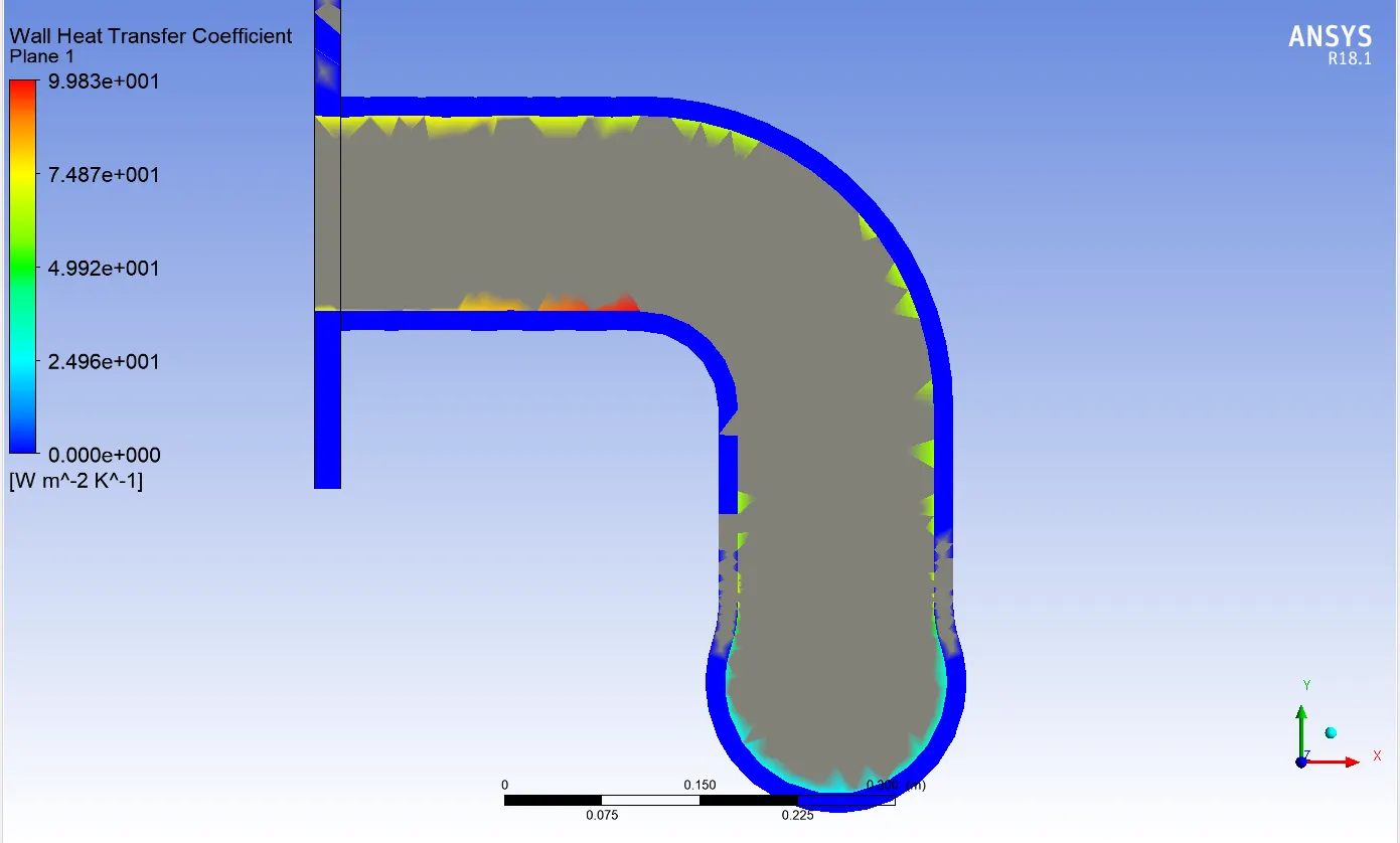
The internal solid wall Heat Transfer coefficient is 99 w/m^2*k.

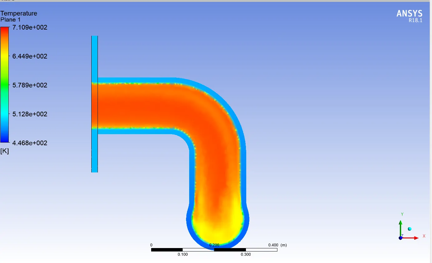
Refined Mesh:

cell counts=4,82,679 and Element size =10mm

Temperature streamline:

Temperature lowers at the throat due to high Heat Transfer rate.

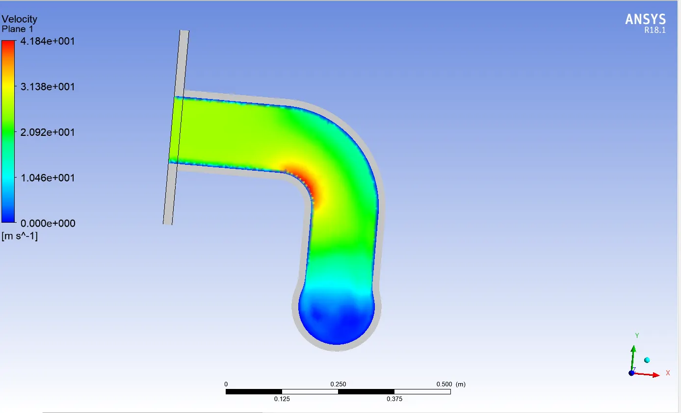
Velocity Streamline:

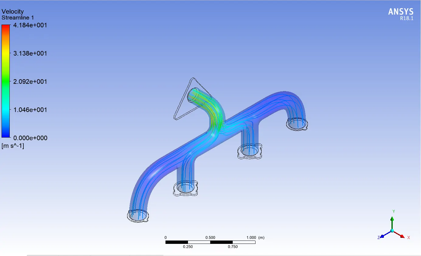
The Velocity at the throat increases due to incoming gases from all the four inlet.

Temperature at the Exit port throat:

Velocity at the Throat:

Heat Transfer coefficient of inner solid Wall:

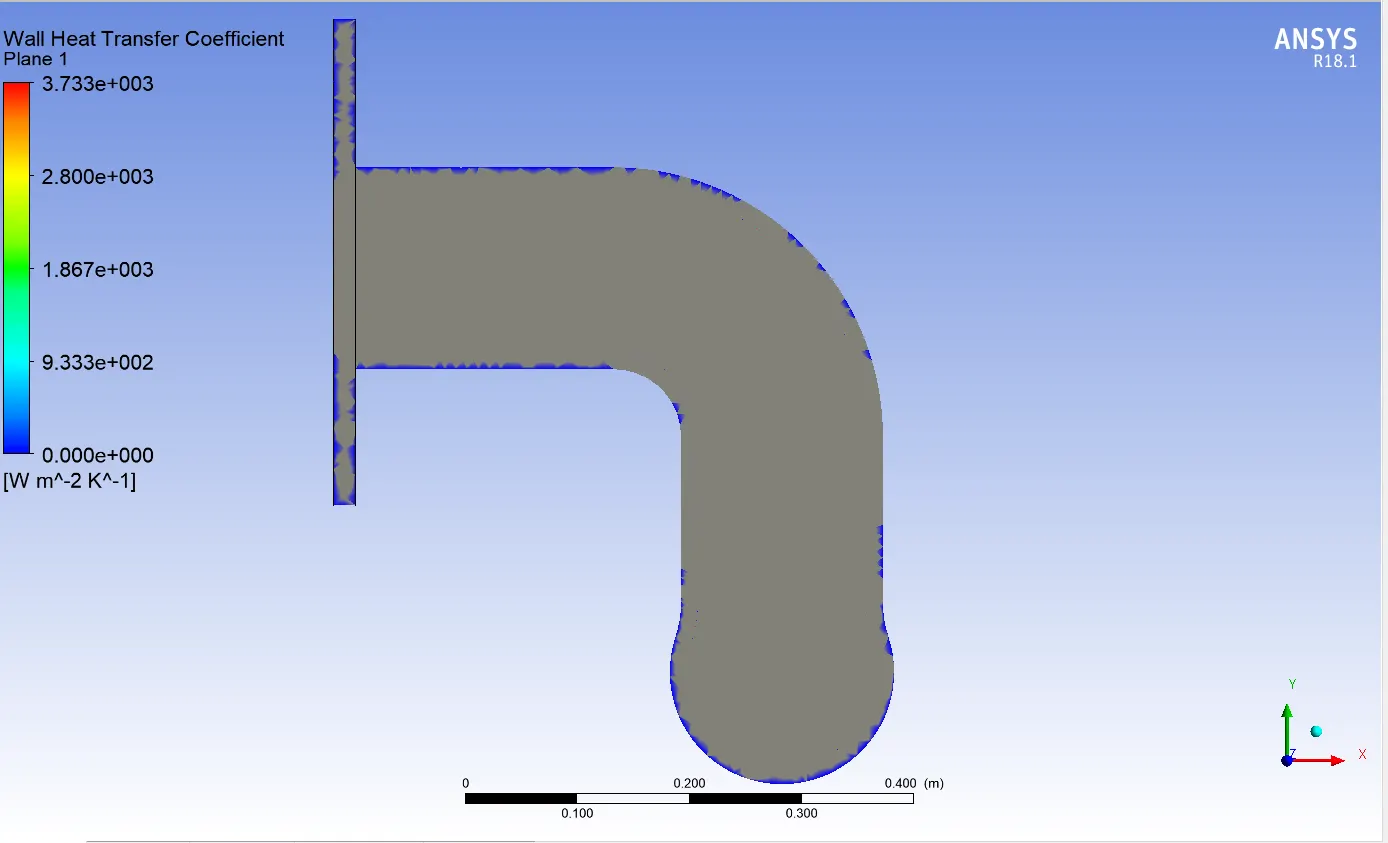
The internal solid wall Heat Transfer coefficient is 905.833 w/m^2*k.

Comparison between Baseline and refined Mesh:

Parameters at the throat of the exit pipe	Baseline Mesh	Refined Mesh
Velocity (m/s)	37.283	41.052
Temperature (Kelvin)	701	710
Heat Transfer coefficient (w/(m^2)k)	99.833	905.69
Cells count	1,46,312	4,82,679

Conclusion:

1) As the Velocity increases, the Heat transfer rate also increases and hence lowers the temperature at the throat of the exit pipe.

In Refined Mesh, there is uniform Velocity and Temperature distribution at throat than Baseline Mesh.

3) The Wall Heat Transfer coefficient of refined Mesh is almost accurate but in Baseline Mesh HTC is very less, i.e highly inaccurate. However there no such large difference between Velocity and temperature value of both the Mesh.

4) As cell counts of refined Mesh is more hence Computation time is also increased.