Evaluating a Function and Comparison of Various Suspension systems using Simulink

Aim: To compare and study the results of various suspension systems using Simulink.

Objectives:

1. Evaluate and plot the given function using Simulink.

2. Comparision of various suspension systems.

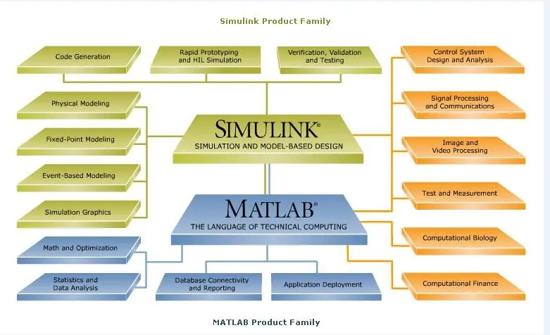
Simulink: Simulink is a MATLAB-based graphical programming environment for modeling, simulating and analyzing multidomain dynamic systems. Its primary interface is a graphical block diagramming tool and a customizable set of block libraries. It offers tight integration with the rest of the MATLAB environment and can either drive MATLAB or be scripted from it. Simulink is widely used in automatic control and digital signal processing for multidomain simulation and model-based design.

EVALUATE AND PLOT THE GIVEN FUNCTION USING SIMULINK

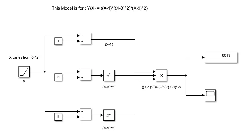
Given Function: Y(x) = (x-1)*(x-3)^2*(x-9)^2

Simulink Model:

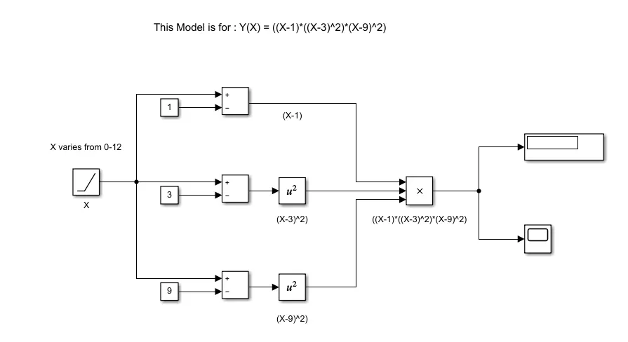
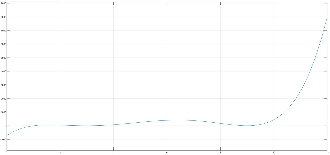
For plotting the function we are varying the 'x' value from 0-12.

Blocks Used:

Ramp: The Ramp block generates a signal that starts at a specified time and value and changes by a specified rate. The block's Slope, Start time, and Initial output parameters determine the characteristics of the output signal. All must have the same dimensions after scalar expansion.

Constant:

The Constant block generates a real or complex constant value signal. Use this block to provide a constant signal input. The block generates scalar, vector, or matrix output, depending on:

The output of the block has the same dimensions and elements as the Constant value parameter. If you specify for this parameter a vector that you want the block to interpret as a vector, select the Interpret vector parameters as 1-D check box. Otherwise, if you specify a vector for the Constant value parameter, the block treats that vector as a matrix.

Subtract:

The Sum block performs addition or subtraction on its inputs. The Add, Subtract, Sum of Elements, and Sum blocks are identical blocks. This block can add or subtract scalar, vector, or matrix inputs. It can also collapse the elements of a signal and perform a summation.

You specify the operations of the block with the List of signs parameter with plus (+), minus (-), and spacer (|).

The Sum block first converts the input data type to its accumulator data type, then performs the specified operations. The block converts the result to its output data type using the specified rounding and overflow modes.

Square: For squaring the solved equation.

Product:

The Product block outputs the result of multiplying two inputs: two scalars, a scalar and a nonscalar, or two nonscalars that have the same dimensions. The default parameter values that specify this behavior are:

Display:

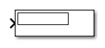
The Display block connects to a signal in your model and displays its value during simulation. You can configure the appearance and format of the Display block to make intuitive sense for the value it displays. You can edit the parameters of the Display block during simulation. The Display block can display complex, vector, and 2-D matrix signals. Use the Display block with other dashboard blocks to build an interactive dashboard of controls and indicators for your model.

Scope:

The Scope is optimized for general time-domain simulation. For a side-by-side comparison

Flow Process:

1. Initially the 'x' value is taken and sent to (x-1),(x-3) and (x-9) blocks to solve the constants.

2. Then the (x-3) and (x-9) block values are squared.

3. Then the values from (x-1),(x-3)^2 and (x-9)^2 blocks are sent to product block for multiplication.

4. Then the output is taken as display for showing the evaluated value and scope block for tracing the changes in the function when 'x' value changes.

5. All the above steps are run like a loop till 'x' value reaches the desired run seconds given by the user.

Verification:

Always the simulink displays the last timer value '12' evaluation for the function.

So,

X=12

Now,

Y(x) = (x-1)*(x-3)^2*(x-9)^2

Y(12) = (12-1)*(12-3)^2*(12-9)^2

Y(12) = (11)*((9)^2)*((3)^2)

Y(12) = 11*81*9

Y(12) = 8019

Output:

COMPARISION OF VARIOUS SUSPENSION SYSTEM USING SIMULINK

Simulink Model:

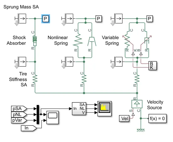
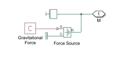
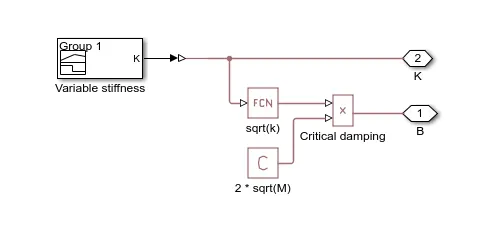
Testbed containing three sets of springs and dampers excited by the same oscillating velocity source. The first uses the Shock Absorber block and includes linear stiffness and damping. Optional friction and hard stops are not used. The second shock absorber uses a Nonlinear Translational Spring and a Nonlinear Translational Damper specified by symmetric polynomials. The third uses a Variable Translational Spring and Variable Translational Damper. The spring constant is varied during the simulation using open loop control and the damping coefficient adjusts to ensure critical damping is achieved. Closed loop control can be added to simulate an adaptive suspensionsystem.

Model Flow:

1. Initially we provide the velocity source to the tire spring and then it gets tranferred through the un-sprung mass.

2. From the un-sprung mass, it gets passed to sprung mass via spring and damper arrangements. The damping co-efficient (B) and spring constant is varied for variable spring suspension system.

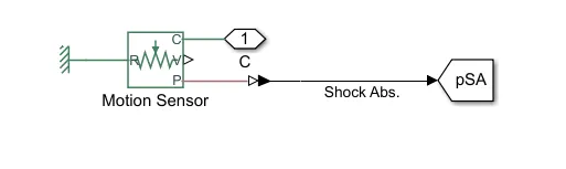
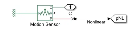
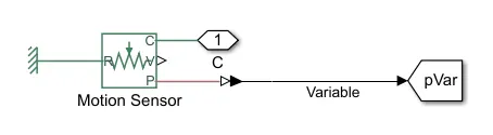
3. The motion sensor is connected to capture the movement and position of the spring during change in velocity.

Question & Answers:

1. What is the objective of the simulation? what are the similarities and differences between the three systems understudy?

The term simulation refers to the use and development of a model. A model is a theoretical representation of a reality. A disaster simulation is an exercise in which a model is developed representing an actual situation: an earthquake, hurricane, or other type of disaster, along with the relevant decisions.

Principal features of simulation:

1) Simulation is a technique oriented toward active participation by instructor and participants. It also represents an approach or point of entry for providing training in a given situation

2) It is generally a problem situation and therefore useful in the interdisciplinary development of the teaching-learning process.

3) It is essentially a dynamic technique which is based on changing situations and requires flexibility in thought and response, which must be adapted to whatever circumstances exist at a given time.

During a simulation exercise, the participants are expected to make decisions in situations that change whenever new information is received.

Some Objectives of a simulation Exercise

1) Present a simplified abstraction of the essential elements of a situation;

2) Make explicit the essential relations and fundamental interactions in a situation;

3) Move the time variable ahead at an accelerated speed so that the implications arising from action taken in a dynamic situation may be clearly experienced;

4) Place the participant in a pressure situation, so that he feels the direct impact of decision-making;

5) Offer an opportunity to participate in the teaching-learning process based on a self-teaching approach.

There is no question but that one of the most significant advantages of simulation is its ability to speed up the passage of time. This is a fundamental characteristic that will enable participants to make decisions on situations that normally would develop over a longer period of time.

To Provide certain range of velocity input and analyze the sprung mass position during vibrations in all the three different types of spring mass arrangements.

Three Damping Systems:

In this model we are using three different arrangement of spring and damper,

1. Shock Absorber:

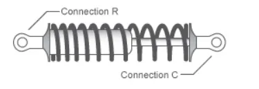
The Shock Absorber block represents a spring-damper system commonly used to dampen vibration in mechanical systems. An internal force acts between ports R and C. This force is the sum of spring stiffness, damping, Coulomb friction, and hard-stop contributions. All force contributions are optional.

2. Non-liner translational spring and damper:

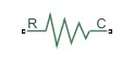
Models a nonlinear translational spring.

If Parameterization is set to By polynomial, force, F, is calculated as F = k1 * x + sign(x) * k2 * x^2 ... + k5 * x^5, where k1 through k5 are the first through fifth-order coefficients, and x is the current deformation. The unit specified is the unit of k1.

If Parameterization is set to By table lookup, force is calculated using the tabulated values of force and deformation. The force must be zero when the deformation is zero.

Connections R and C are mechanical translational conserving ports.

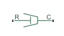
Models a nonlinear translational damper.

If Parameterization is set to By polynomial, force, F, is calculated as F = b1 * v + sign(v) * b2 * v^2 ... + b5 * v^5, where b1 through b5 are the first through fifth-order coefficients, and v is the velocity of port R minus the velocity of port C. The unit specified is the unit of b1.

If Parameterization is set to By table lookup, force is calculated using the tabulated values of force and velocity. The force must be zero when the velocity is zero.

Connections R and C are mechanical translational conserving ports.

3. Variable translational spring and damper:

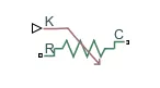
Models a linear variable translational spring. Force, F, is calculated as F = K * x, where K is the physical signal input and x is the current deformation. The Minimum spring rate prevents non-physical negative K values.

Connections R and C are mechanical translational conserving ports. The block positive direction is from port R to port C. This means that the force is positive if it acts in the direction from R to C.

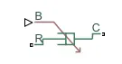
Models a linear variable translational damper. Force, F, is calculated as F = B * v, where B is the physical signal input and v is the relative velocity between connections R and C. The Minimum damping coefficient prevents non-physical negative B values.

Connections R and C are mechanical translational conserving ports. The block positive direction is from port R to port C. This means that the force is positive if it acts in the direction from R to C.

2. What are your observations from the results?

The observations after simulating the model is the vibrations of the three systems and the position of the sprung mass during the vibration frequency variation.

Result 1:

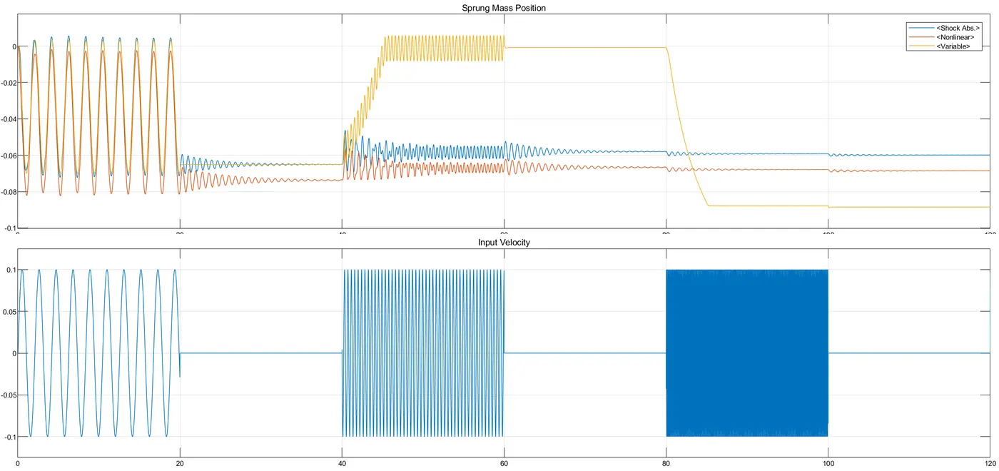
In this plot we can observe that the position of the sprung mass during the change in velocity and vibration of the spring. Initially the spring gets vibrated during the input velocity and gets damped out by the damper.

Till time (t=20sec) the vibration of all the three systems are same and then gets damped out.

From time (t=20 to t=60sec) the variable spring vibrates and damps out. But the suspension and linear one vibrates till (t=70sec) and then gets damped out.

Further there are very small vibrations in between (t=80 to t=100sec) interval in suspension and linear one and then gets damped out.

Result 2:

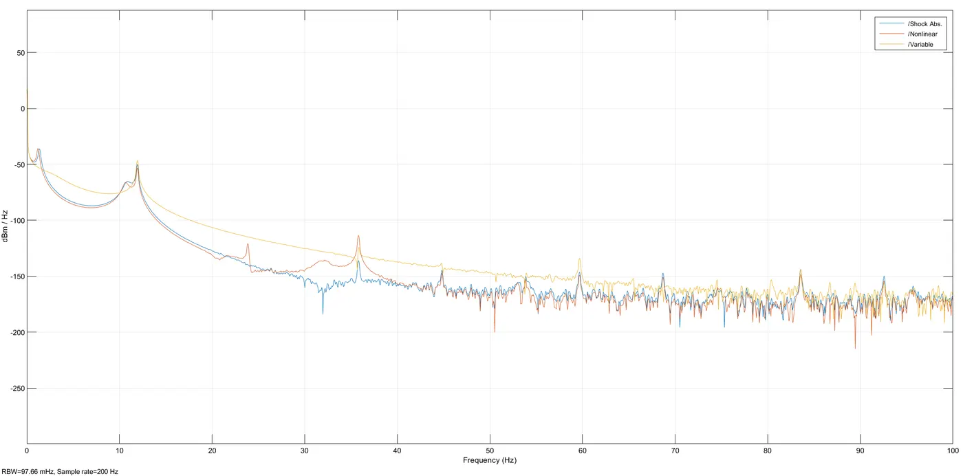
From this plot we can observe that the vibration frequency (Hz) of the springs in all the three systems from the noise (dB) during the change in input velocity.

3. How the oscillating velocity source is created?

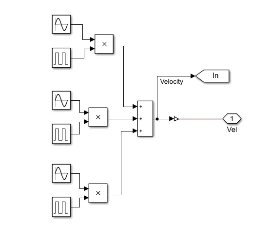
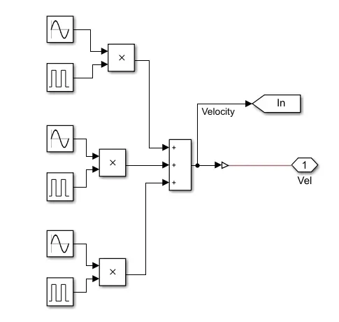
The oscillating velocity is created using sine wave and pulse generator block

Sine Wave: The Sine Wave block outputs a sinusoidal waveform. The block can operate in time-based or sample-based mode.

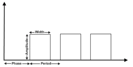
Pulse generator: The Pulse Generator block generates square wave pulses at regular intervals. The block waveform parameters, Amplitude, Pulse Width, Period, and Phase delay, determine the shape of the output waveform. The following diagram shows how each parameter affects the waveform.

Model File:

https://drive.google.com/file/d/1QcG4h2SLkIfKR8vsa3ixtob6PF7laqVv/view?usp=sharing

Reference:

https://in.mathworks.com/help/physmod/sdl/examples/suspension-system-comparison.html?s_tid=srchtitle

Conclusion: From the above simulation we are able to solve a function using Simulink and simulate the three suspension system to understand their behavior (Vibration, damping & frequency) during change in velocity.