Genetic Algorithm to calculate the Global Maxima of Stalagmite Function using Matlab.

Classical Algorithm	Genetic Algorithm
Generates a single point at each iteration. The sequence of points approaches an optimal solution.	Generates a population of points at each iteration. The best point in the population approaches an optimal solution.
Selects the next point in the sequence by a deterministic computation.	Selects the next population by computation which uses random number generators.

A genetic algorithm is a search heuristic that is inspired by Charles Darwin’s theory of natural evolution. This algorithm reflects the process of natural selection where the fittest individuals are selected for reproduction in order to produce offspring of the next generation.

Nation of Natural Selection

The process of natural selection starts with the selection of fittest individuals from a population. They produce offspring which inherit the characteristics of the parents and will be added to the next generation. If parents have better fitness, their offspring will be better than parents and have a better chance at surviving. This process keeps on iterating and at the end, a generation with the fittest individuals will be found.

This notion can be applied for a search problem. We consider a set of solutions for a problem and select the set of best ones out of them.

Five phases are considered in a genetic algorithm.

1. Initial population
2. Fitness function
3. Selection
4. Crossover
5. Mutation

Global Optimization :

Optimization is the process of finding the point that minimizes a function. More specifically:

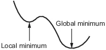
Generally, Optimization Toolbox solvers find a local optimum. (This local optimum can be a global optimum.) They find the optimum in the basin of attraction of the starting point. For more information, see Basins of Attraction.

In contrast, Global Optimization Toolbox solvers are designed to search through more than one basin of attraction. They search in various ways:

STALAGMITE :

A stalagmite is a type of rock formation that rises from the floor of a cave due to the accumulation of material deposited on the floor from ceiling drippings. Stalagmites are typically composed of calcium carbonate, but may consist of lava, mud, peat, pitch, sand, sinter and amberat (crystallized urine of pack rats).

Stalagmite Function :

It is a mathematical model that helps to generate local minima and maxima, it is a three-dimensional function and the way the function is designed is that it has a lot of local maxima or minima or one global maxima or minima.

The function that is used to obtain 3D model of stalagmite model is,

Where,

Syntax of GA

The 'ga' syntax in Matlab is used to find the minimum of a function using a genetic algorithm. There are several ways to define the 'ga' function depending on the problem being solved. The syntax used for this study is shown below.

x = ga(fun,nvars) finds a local unconstrained minimum, x, to the objective function, fun. nvars is the dimension (number of design variables) of fun.

x = ga(fun,nvars,A,b) finds a local minimum x to fun, subject to the linear inequalities A*x ≤ b. ga evaluates the matrix product A*x as if x is transposed (A*x').

x = ga(fun,nvars,A,b,Aeq,beq) finds a local minimum x to fun, subject to the linear equalities Aeq*x = beq and A*x ≤ b. (Set A=[] and b=[] if no linear inequalities exist.) ga evaluates the matrix product Aeq*x as if x is transposed (Aeq*x').

x = ga(fun,nvars,A,b,Aeq,beq,lb,ub) defines a set of lower and upper bounds on the design variables, x, so that a solution is found in the range lb ≤ x ≤ ub. (Set Aeq=[] and beq=[] if no linear equalities exist.)

x = ga(fun,nvars,A,b,Aeq,beq,lb,ub,nonlcon) subjects the minimization to the constraints defined in nonlcon. The function nonlcon accepts x and returns vectors C and Ceq, representing the nonlinear inequalities and equalities respectively. ga minimizes the fun such that C(x) ≤ 0 and Ceq(x) = 0. (Set lb=[] and ub=[] if no bounds exist.)

x = ga(fun,nvars,A,b,Aeq,beq,lb,ub,nonlcon,options) minimizes with the default optimization parameters replaced by values in options. (Set nonlcon=[] if no nonlinear constraints exist.) Create options using optimoptions.

x = ga(fun,nvars,A,b,[],[],lb,ub,nonlcon,IntCon) or x = ga(fun,nvars,A,b,[],[],lb,ub,nonlcon,IntCon,options) requires that the variables listed in IntCon take integer values.

x = ga(problem) finds the minimum for problem, where problem is a structure.

[x,fval] = ga(___), for any previous input arguments, also returns fval, the value of the fitness function at x.

[x,fval,exitflag,output] = ga(___) also returns exitflag, an integer identifying the reason the algorithm terminated, and output, a structure that contains output from each generation and other information about the performance of the algorithm.

[x,fval,exitflag,output,population,scores] = ga(___) also returns a matrix population, whose rows are the final population, and a vector scores, the scores of the final population.

GENETIC ALGORITHM IN MATLAB :

In Matlab, Genetic Algorithm (GA) is used to global minima for hign non-linear problems. The syntax used in this program are,

SYNTAX 1 : [x,fval] = ga(fun,nvars)

SYNTAX 2 : x = ga(fun,nvars,A,b,Aeq,beq,lb,ub)

SYNTAX 3 : options = optimoptions(Solver Name)

SYNTAX 4 : options = optimoptions(Solver Name,Name,Solver)

SYNTAX 5 : x = ga(fun,nvars,A,b,Aeq,beq,lb,ub,nonlcon,options)

Matlab Program :

Stalagmite Function Code

function[f] = stalagmite_func(input_vector)
x = input_vector(1);
y = input_vector(2);

term1 = (sin((5.1*pi*x)+0.5))^6;
term2 = (sin((5.1*pi*y)+0.5))^6;
term3 = exp(-4*log(2)*((x-0.0667)^2)/0.64);
term4 = exp(-4*log(2)*((y-0.0667)^2)/0.64);

f = -(term1*term2*term3*term4);
end

Steps undertaking during programming.

1. The complier start the program.

2. Using function code the values for X & Y are imported from the main code.

3. Then the variables for X & Y are assigned respectively.

4. Next all the terms in the above equation are being solved.

5. Finally all the four terms are multiplied in the sequence of above equation to obtaining stalagmite data points.

6. Function code ends.

7. The function code used below is commom for all three studies performed to obtain the Global Maxima

Study 1 - Statistical Behaviour Without Bounds:

%*********** Study1 - Statistical Behaviour without Bounds****************
clear all
close all
clc

% Defining the search space
x = linspace(0,0.6,150);
y = linspace(0,0.6,150);
n = 50;     % Number of iterations

[xx, yy] = meshgrid(x,y);

% Evaluating Stalagmite Function
for i = 1:length(xx)
    for j = 1:length(yy)
        input_vector(1) = xx(i,j);
        input_vector(2) = yy(i,j);
        f(i,j) = stalagmite_func(input_vector);
    end
end

tic
% Case1 - Stastical Behaviour
for k = 1:n
    [inputs,fopt(k)] = ga(@stalagmite_func,2);
    xopt(k) = inputs(1);
    yopt(k) = inputs(2);
end

study1_time = toc
subplot(2,1,1)
hold on
surf(xx,yy,-f)
shading interp
grid on

plot3(xopt,yopt,-fopt,'Marker','o','MarkerFaceColor','r')
xlabel('X Values')
ylabel('Y Values')
zlabel('Function Values')
title('Unbounded Inputs')
subplot(2,1,2)
plot(-fopt)
xlabel('Iterations')
ylabel('fopt')
title('Statistical Behaviour')

Steps undertaking during programming.

1. The complier start the program.

2. Defining the search space for both x & y and defining the number of iterations.

3.Using "meshgrid" command 2D array is generated.

4. Evaluating stalagmite function and defined length of x & y calculated and store in i , j variables respectively.

5. Storing the x & y data to the stalagmite function.

6. Using genetic algorithm to predict global maxima in no boundary conditions and storing all the optimum values during iterations.

7. Looping statement ends for both i,j variables.

8. Then using "surf" command to plot 3D model for the stalagmite function.

9. Using "shading interp" command to remove grid lines on 3D plot.

10. Plot the stalagmite model with respective variables and RGB triplate for 3D plot.

11. Defining x & y axis and defining title.

12. Run the program and get the below result.

Study 2 - Statistical Behaviour With Bounds:

%*********** Study2 - Statistical Behaviour with Bounds****************
clear all
close all
clc

% Defining the search space
x = linspace(0,0.6,150);
y = linspace(0,0.6,150);
n = 50;     % Number of iterations

[xx, yy] = meshgrid(x,y);

% Evaluating Stalagmite Function
for i = 1:length(xx)
    for j = 1:length(yy)
        input_vector(1) = xx(i,j);
        input_vector(2) = yy(i,j);
        f(i,j) = stalagmite_func(input_vector);
    end
end

tic
% Case1 - Stastical Behaviour
for k = 1:n
    [inputs,fopt(k)] = ga(@stalagmite_func,2,[],[],[],[],[0;0],[0.6;0.6]);
    xopt(k) = inputs(1);
    yopt(k) = inputs(2);
end

study1_time = toc
subplot(2,1,1)
hold on
surf(xx,yy,-f)
shading interp
grid on

plot3(xopt,yopt,-fopt,'Marker','o','MarkerFaceColor','r')
xlabel('X Values')
ylabel('Y Values')
zlabel('Function Values')
title('Bounded Inputs')
subplot(2,1,2)
plot(-fopt)
xlabel('Iterations')
ylabel('fopt')
title('Statistical Behaviour')

Steps undertaking during programming.

1. The complier start the program.

2. Defining the search space for both x & y and defining the number of iterations.

3.Using "meshgrid" command 2D array is generated.

4. Evaluating stalagmite function and defined length of x & y calculated and store in i , j variables respectively.

5. Storing the x & y data to the stalagmite function.

6. Using genetic algorithm to predict global maxima in boundary conditions and storing all the optimum values during iterations.

7. Genetic Algorithm finds the optimum values within the given boundary conditions.

8. Looping statement ends for both i,j variables.

9. Then using "surf" command to plot 3D model for the stalagmite function.

10. Using "shading interp" command to remove grid lines on 3D plot.

11. Plot the stalagmite model with respective variables and RGB triplate for 3D plot.

12. Defining x & y axis and defining title.

13. Run the program and get the below result.

Study 3 - Statistical Behaviour With Bounds and A Larger Population:

%***Study3 - Statistical Behaviour with Bounds & A Larger Population****
clear all
close all
clc

% Defining the search space
x = linspace(0,0.6,150);
y = linspace(0,0.6,150);
n = 50;     % Number of iterations

[xx, yy] = meshgrid(x,y);

% Evaluating Stalagmite Function
for i = 1:length(xx)
    for j = 1:length(yy)
        input_vector(1) = xx(i,j);
        input_vector(2) = yy(i,j);
        f(i,j) = stalagmite_func(input_vector);
    end
end

tic
% Case1 - Stastical Behaviour
options = optimoptions('ga')
options = optimoptions(options,'PopulationSize',300);
for k = 1:n
    [inputs,fopt(k)] = ga(@stalagmite_func,2,[],[],[],[],[0;0],[0.6;0.6],[],[],options);
    xopt(k) = inputs(1);
    yopt(k) = inputs(2);
end

study1_time = toc
figure(1)
subplot(2,1,1)
hold on
surf(xx,yy,-f)
shading interp
grid on

plot3(xopt,yopt,-fopt,'Marker','o','MarkerFaceColor','r')
xlabel('X Values')
ylabel('Y Values')
zlabel('Function Values')
title('Bounded Inputs with Larger Population')
subplot(2,1,2)
plot(-fopt)
xlabel('Iterations')
ylabel('fopt')
title('Statistical Behaviour')

Steps undertaking during programming.

1. The complier start the program.

2. Defining the search space for both x & y and defining the number of iterations.

3.Using "meshgrid" command 2D array is generated.

4. Evaluating stalagmite function and defined length of x & y calculated and store in i , j variables respectively.

5. Storing the x & y data to the stalagmite function.

6. Modifying the population size with boundary conditions using "optimoptions" command and considered 300 as population size.

7. Genetic Algorithm syntex finds the optimum values within the given boundary conditions.

8. Looping statement ends for both i,j variables.

9. Then using "surf" command to plot 3D model for the stalagmite function.

10. Using "shading interp" command to remove grid lines on 3D plot.

11. Plot the stalagmite model with respective variables and RGB triplate for 3D plot.

12. Defining x & y axis and defining title.

13. Run the program and get the below result.

Output :

In this code we obtained the Global Maxima value from the function and its achieved by increasing the population size.

Best Fit of X and Y Values respectively = 0.06683 and 0.06683

Global Maxima = 1

Errors:

No complicated errors occured while running the Matlab Program.

CONCLUSION :

In the comparision of all three studies like Stastical behaviour without boundary conditions,with boundary conditions and with boundary conditions with a larger population, the third one is best for obtaining the global maxima.

References:

https://en.wikipedia.org/wiki/Genetic_algorithm

https://towardsdatascience.com/introduction-to-genetic-algorithms-including-example-code-e396e98d8bf3

https://in.mathworks.com/help/gads/what-is-global-optimization.html

https://in.mathworks.com/help/gads/ga.html