Developing Code using MATLAB for Error Comparison of different numerical schemes

AIM—

• Derivation of 4^th order approximation for the second order derivative using

1. Central difference
2. Skewed right side difference
3. Skewed left side difference

• Error Comparison of numerical scheme developed by above numerical method

THEORY

For same order of accuracy , increasing the order of derivative by one order requires the inclusion of an additional point . Thus a general formula can be written If ‘p’ is the order of the derivative being evaluated, q is the accuracy of discretization and n is the no of adjacent points used in the discretization, then

n = p+q-1 (For Central difference)

n = p+q (For Skewed Scheme)

N.B- The above formula is only valid for uniform grid spacing

Central difference

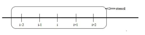
Assuming uniform grid spacing and using above formula we can write 4^th order approximation for central difference in following way by using Taylor table---

`f''(x) = af_(i-2)+bf_(i+1)+cf_(i)+df_(i+1)+ef_(i+2)`-------------------(1)

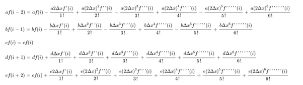
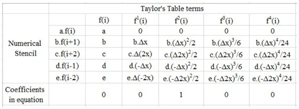
Arranging the co-efficient terms of the Taylor table and equating with equation (1) following equations can be obtained.

`a+b+c+d+e = 0`

`-2a-b+d+2e =0`

`((4a)/2)+b/2+d/2+(4e)/2=1`

`(-8a)/6-b/6+d/6+(8e)/6=0`

`(16a)/24+b/24+d/24+(16e)/24=0`

By Solving above co-efficient equation by Matrix inversion method ---

u = T^-1V

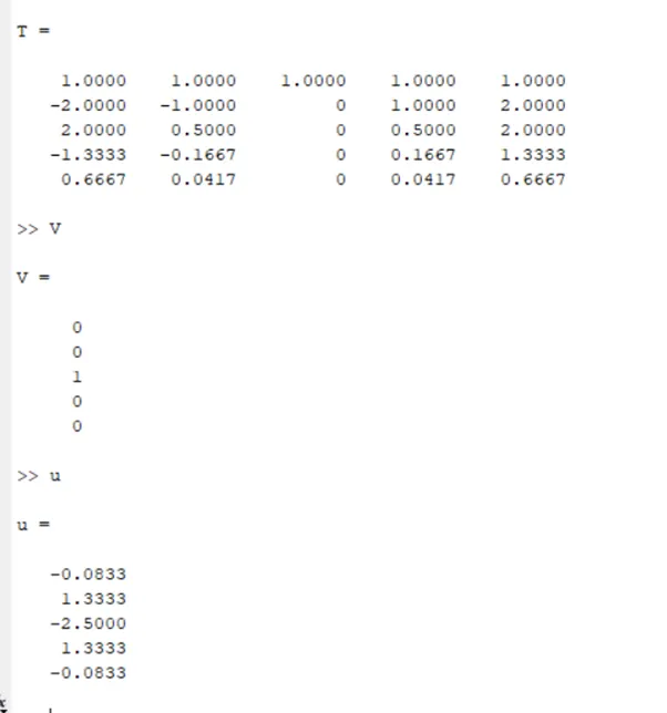
Rewriting equation (1), we get---

`f''(x) = (-.0833f_(i-2)+1.3333f_(i+1)+2.5f_(i)+1.3333f_(i+1)-0.0833f_(i+2))/(dx)^2`

Skewed right side difference

In skewed right side difference scheme, all the nodes in numerical stencils are towards the right side.

Assuming uniform grid spacing and using above formula we can write 4^th order approximation for Skewed right difference in following way by using Taylor table---

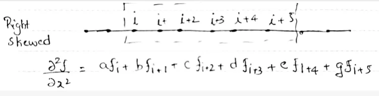
`f''(x) = af_(i)+bf_(i+1)+cf_(i+2)+df_(i+3)+ef_(i+4)+f_(i+5)`---------------(2)`

Taylor Table

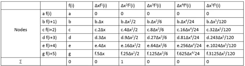
Arranging the co-efficient terms of the Taylor table and equating with equation (2) following equations can be obtained.

`a+b+c+d+e +g= 0`

`b+2c+3d+4e+5g = 0`

`b/2+(4c)/2+(9d)/2+(16e)/2+(25g)/2=1`

`b/6+(8c)/6+(27d)/6+(64e)/6+(125g)/6=0`

`b/24+(16c)/24+(81d)/24+(256e)/24+(625g)/24=0`

`b/120+(32c)/120+(243d)/120+(1024e)/120+(3125g)/120=0`

Solving the above equations in matlab---

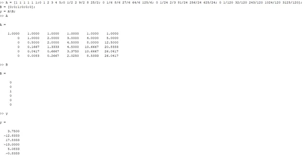
Rewriting equation (2), we get---

`f''(x) = 3.7500f_(i)-12.8333f_(i+1)+17.8333f_(i+2)-13f_(i+3)+5f_(i+4)-0.8333_(i+5)`

Skewed Left side difference

In skewed left side difference scheme, all the nodes in numerical stencils are towards the left side.

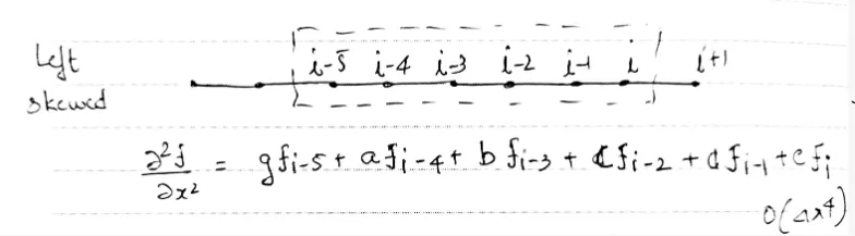
`f''(x) = af_(i)+bf_(i-1)+cf_(i-2)+df_(i-3)+ef_(i-4)+f_(i-5)`-----------(3)

Assuming uniform grid spacing and using above formula we can write 4^th order approximation for Skewed left difference in following way by using Taylor table---

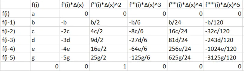
Arranging the co-efficient terms of the Taylor series and equating with equation (3) following equations can be obtained.

`a+b+c+d+e +g= 0`

`-b-2c-d-4e-5g = 0`

`b/2+(4c)/2+(9d)/2+(16e)/2+(25g)/2=1`

`-b/6-(8c)/6-(27d)/6-(64e)/6-(125g)/6=0`

`b/24+(16c)/24+(81d)/24+(256e)/24+(625g)/24=0`

`-b/120-(32c)/120-(243d)/120-(1024e)/120-(3125g)/120=0`

Solving above equations in MATLAB----

% Skewed left augmented matrix

P = [1 1 1 1 1 1;0 -1 -2 -3 -4 -5;0 1/2 2 9/2 8 25/2; 0 -1/6 -8/6 -27/6 -64/6 -125/6; 0 1/24 2/3 81/24 256/24 625/24; 0 -1/120 -32/120 -243/120 -1024/120 -3125/120];
Q = [0;0;1;0;0;0];

%co-efficients
S = PQ;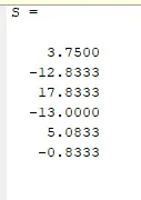

MATLAB CODE-:

close all
clear all
clc
% taylor table
% f' = exp(x).cos(x)
% skewed right side difference
% Skewed left augmented matrix

P = [1 1 1 1 1 1;0 -1 -2 -3 -4 -5;0 1/2 2 9/2 8 25/2; 0 -1/6 -8/6 -27/6 -64/6 -125/6; 0 1/24 2/3 81/24 256/24 625/24; 0 -1/120 -32/120 -243/120 -1024/120 -3125/120];
Q = [0;0;1;0;0;0];

%co-efficients
S = PQ;


% skewed right augmented matrix
A = [1 1 1 1 1 1;0 1 2 3 4 5;0 1/2 2 9/2 8 25/2; 0 1/6 8/6 27/6 64/6 125/6; 0 1/24 2/3 81/24 256/24 625/24; 0 1/120 32/120 243/120 1024/120 3125/120];
B = [0;0;1;0;0;0];
y = AB;

% central difference
% augmented matrix
T = [1 1 1 1 1;-2 -1 0 1 2; 2 1/2 0 1/2 2; -8/6 -1/6 0 1/6 8/6;16/24 1/24 0 1/24 16/24];
V = [0;0;1;0;0];
u = TV;
% giving input
x = pi/4;
dx = linspace(pi/40,pi/40000,10);
% analytical solution
analyt_ans = -2*(exp(x)*sin(x));
% for loop
for i = 1:length(dx)
%skewed right forward scheme

skd_rht (i)= ((y(1)*((exp(x))*(cos(x))))+(y(2)*((exp(x+(dx(i))))*(cos(x+(dx(i))))))...
    +(y(3)*((exp(x+(2*(dx(i)))))*(cos(x+(2*(dx(i)))))))+(y(4)*((exp(x+(3*(dx(i)))))*(cos(x+(3*(dx(i)))))))...
    + (y(5)*((exp(x+(4*(dx(i)))))*(cos(x+(4*(dx(i)))))))+(y(6)*((exp(x+(5*(dx(i)))))*(cos(x+(5*(dx(i))))))))/(dx(i))^2;

skd_lft (i)= ((S(1)*((exp(x))*(cos(x))))+(S(2)*((exp(x-(dx(i))))*(cos(x-(dx(i))))))+(S(3)*((exp(x-(2*(dx(i)))))*(cos(x-(2*(dx(i)))))))...
    +(S(4)*((exp(x-(3*(dx(i)))))*(cos(x-(3*(dx(i)))))))+ (S(5)*((exp(x-(4*(dx(i)))))*(cos(x-(4*(dx(i)))))))+...
    (S(6)*((exp(x-(5*(dx(i)))))*(cos(x-(5*(dx(i))))))))/(dx(i))^2;
cntrl_diff(i) = ((u(1)*((exp(x-(2*dx(i))))*(cos(x-(2*dx(i))))))+(u(2)*((exp(x-(dx(i))))*(cos(x-(dx(i))))))...
    +(u(3)*((exp(x))*(cos(x))))+(u(4)*((exp(x+((dx(i)))))*(cos(x+((dx(i)))))))...
    + (u(5)*((exp(x+(2*(dx(i)))))*(cos(x+(2*(dx(i))))))))/(dx(i))^2;



end

error_left = abs(skd_lft-analyt_ans);
error_right = abs(skd_rht-analyt_ans);
error_central = abs(cntrl_diff-analyt_ans);
loglog(dx,error_left,'Linewidth',1.5)
hold on
loglog(dx,error_right,'Linewidth',1.5)
hold on
loglog(dx,error_central,'Linewidth',1.5)
hold on
loglog(dx,analyt_ans,'Linewidth',1.5)
legend('skewd_left(oh4)', 'skewed_right(oh4)', 'central diff (oh4)', 'Ana;ytical Solution')

OBSERVATION

The given function can yield analytical solution as-

`-2*(exp(x)*sin(x));`

We now consider various approximation to the second derivative with step size of `deltax=.0785`

CENTRAL

SKEWED RIGHT

Skewed left

ERROR

CENTRAL

SKEWED RIGHT

Skewed left

Results are tabulated below

F’’(x) (Exact)	-3.1018
CD4	-3.1018
Five point forward	-3.1023
Five point backward	-3.1020

It seen that the error is unacceptable in the case of both Skewed FDS and Skewed BDS. How ever the estimates that use central difference gives the solution of same order with respect to exact solution. We now change the step size to .0350.

Results are tabulated below

F’’(x) (Exact)	-3.1018
CD4	-3.1018
Five point forward	-3.1018
Five point backward	-3.1018

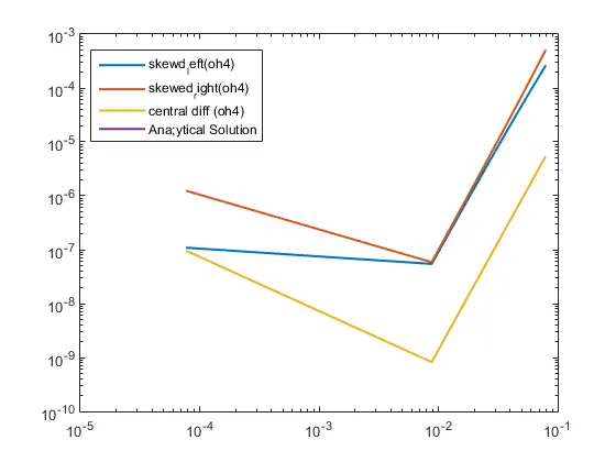
Plot

CONCLUSION

1. We see that the error has moved to the 16^th place after the decimal point in the case of Skewed left, Skewed right and CD₄ Scheme, when grid spacing halved. The MATLAB plot shows error of numerical differentiation formulae for different step sizes using Double precision (16 place after decimal). The figure clearly asserts the importance of order of accuracy. The slope of the error Vs step size plot indicates the order of accuracy of the approximation in the, linear portion. The skewed right of O(h⁴) has has the list slope where as central difference of O(h⁴) has highest slope.
2. Also, It must be noted that the error of the approximation reaches a minimum and then starts increasing with smaller step size. Theoretically, as the step size tends towards zero, the approximation should tend towards exact solution. However this is not the case due to round off errors i.e limited numerical precision of the computer.
3. It can be seen from the graph that 4^th order accurate central scheme gives a better approximation to the true 2^nd derivative, for a coarse grid . For fine grid and rapidly varying solution, it is not necessary that the CD₄ is always better.

4. Skewed scheme are useful at boundaries as CD scheme can not use there.