Drag Force of a Bicyclist
Aim:
The aim is to calculate the drag force against a cyclist and plotting a graph as follows
- Plotting a graph between the Velocity and the Drag Force.
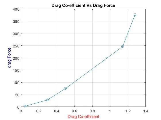
- Plotting a graph between the Drag Co-efficient and the Drag Force.
Theory:
Drag force:
A drag force is the resistance force caused by the motion of a body through a fluid, such as water or air. A drag force acts opposite to the direction of the oncoming flow velocity. This is the relative velocity between the body and the fluid.
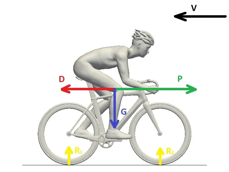
- V the wind direction
- P the propulsion force
- D the aerodynamic drag force
- G the gravity acceleration
- R1, R2 the ground reaction
In the picture above, we can see that the only force preventing the rider from cruising is the aerodynamic drag force (without sloping ground). This is why drag is a very important factor in defining the performance of a bike and why aerodynamicists invest a significant amount of time in optimizing the shape of the bike and the equipment, as well as the rider’s position to achieve maximum performance.
Equations Used:
The Drag Force equation is as follows:
`F_d=1/2 ρAv^2 c_d`
Where
`F_d`=Drag Force in (`kg-m/s^2` )
`ρ` = Density of Air in ( `kg⁄m^3` )
A = Frontal Area in ( `m^2` )
V = Velocity of the Cyclist in ( `m⁄s` )
`c_d` = Drag Coefficient
Procedure:
- For Individual Plotting:
- Plotting the graph between the Velocity and the Drag Force:
- The input values, in this case, are density, Frontal Area, and the Drag Co-efficient of the Cyclist.
%Inputs
c_d=0.8; %Drag Co-efficient
A=0.1; % Area m^2
rho= 1.2; %Density kg/m^3
- The code can be written as a simple line by giving the Velocity values using ‘linspace’.
%For Linearly spaced Velocity values use as below (By uncommenting it)
%Velocity= linspace(0,25,5);
- Taking the number of Velocity Values to give the input of that many velocities.
%For non-linear velocity values, which can be given manually
no_of_Velocities= input("Number of Velocities to be entered: ");- The program is written in a way so that the numbers of velocities are entered and the values are given manually so that the graph is constructed accordingly.
for v= (1:no_of_Velocities)

    Velocity(v)=input('Enter the Velocity: '); %velocity


end
fprintf("The Velocities are:");
disp(Velocity);
drag_force= (1/2)*rho*A.*(Velocity.^2)*c_d;

fprintf("the Drag Forces are: %d kg-m/s^2 n", drag_force);
fprintf('n The Drag Forces are: ');
disp(drag_force);
- The plotting for the graph is written.
%Plotting

plot(Velocity, drag_force)
axis( [0 100 0 200])
title(' Velocity Vs Drag Force', 'fontweight', 'Bold')
xlabel('Velocity')
ylabel('drag Force')
grid on
- Plotting the graph between the Drag Co-efficient and the Drag Force:
- The input values, in this case, are density, frontal area, and the Velocity as the constant. The Drag Coefficient changes as per the shape.
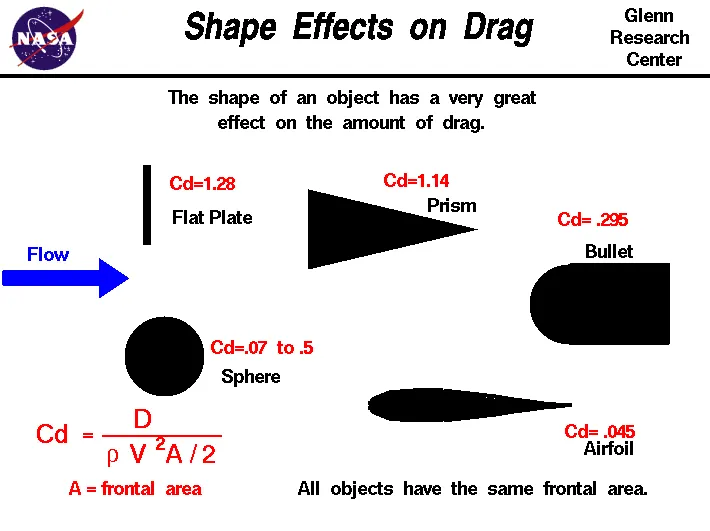
%For Drag Co-efficient Vs Drag Force

%Inputs
A= 0.1;         % Frontal Area in m^2
rho= 1.2;       %Density of Air in kg/m^3
Velocity= 55;   %Velocity of the Cyclist in m/sec
- The code can be written as an array with different drag co-efficient in it.
- The program is written in a way that different drag co-efficient is given as an input so that the drag coefficient can be changed as per requirement.
number_of_Drag_coefficients= input("Number of Drag Co-Efficients to be entered: ");

for c= (1:number_of_Drag_coefficients)

    c_d(c)=input('Enter the Drag Co-efficient: '); %Drag Co-efficient


end

fprintf("The Drag Co-Efficients are: ");
disp(c_d);
drag_force= (1/2)*rho*A*(Velocity^2).*c_d;
fprintf("the Drag Forces are: %d kg-m/s^2n", drag_force);
fprintf("The Drag Forces are: ");
disp(drag_force);- The Plotting of the graph is written below
%Plotting
plot(c_d, drag_force)
title('Drag Co-efficient Vs Drag Force')
xlabel('Drag Co-efficient', 'color', 'r' )
ylabel('Drag Force', 'color', 'b')
grid on- For Combined Plotting:
- The combined plotting might be a bit confusing. In general terms, the Combined type of plotting is to use the 2 sets of array data to get the required output.
- The code runs for each velocity at different Drag Coefficient Values which makes it complex to understand.
- The idea is to give a clear view of Different Velocities with the same amount of Drag Coefficients (Check Reason in the Error Section)
- The Code starts with the input values of the Frontal Area and Density.
%Inputs
A=0.1; % Area m^2
rho= 1.2; %Density kg/m^3
- The code then runs to take the number of Velocities and Drag Coefficients for Calculation.
no_of_Velocities= input("Number of Velocities to be entered: ");
number_of_Drag_coefficients= input("Number of Drag Co-Efficients to be entered: ");- It further takes the input for the value of the velocity and drag coefficients.
for v= (1:no_of_Velocities)

    Velocity(v)=input('Enter the Velocity: ' ); %velocity


end

for c= (1:number_of_Drag_coefficients)

    c_d(c)=input('Enter the Drag Co-efficient: '); %Drag Co-efficient

end
- The Drag force is then calculated for the different velocities and different drag coefficients.
for v = 1: no_of_Velocities
    for c = 1: number_of_Drag_coefficients

        drag_force = (1/2)*rho*A.*(Velocity.^2).*c_d;
    end
end
fprintf("The Drag Co-Efficients are: ");
disp(c_d);
fprintf("The Velocities are:");
disp(Velocity);
fprintf("the Drag Forces are: %d n", drag_force);
- The plotting of the graph is done for both the cases.
%Plotting
figure(1)
plot(Velocity,drag_force, 'Marker', 'o')
title(' Velocity Vs Drag Force', 'fontweight', 'Bold')
xlabel('Velocity')
ylabel('drag Force')
grid on


figure(2)
plot(c_d,drag_force, 'Marker','o')
title('Drag Co-efficient Vs Drag Force')
xlabel('Drag Co-efficient', 'color', 'r' )
ylabel('drag Force', 'color', 'b')
grid on
Code:
The Complete code is written as follows
- For Velocity Vs Drag Force:
clear
close
clc

%Inputs
c_d=0.8; %Drag Co-efficient
A=0.1; % Area m^2
rho= 1.2; %Density kg/m^3

%For Linearly spaced Velocity values use as below (By uncommenting it)
%Velocity= linspace(0,25,5);

%For non-linear velocity values, which can be given manually
no_of_Velocities= input("Number of Velocities to be entered: ");

for v= (1:no_of_Velocities)

    Velocity(v)=input('Enter the Velocity: '); %velocity


end
fprintf("The Velocities are:");
disp(Velocity);
drag_force= (1/2)*rho*A.*(Velocity.^2)*c_d;

fprintf("the Drag Forces are: %d kg-m/s^2 n", drag_force);
fprintf('n The Drag Forces are: ');
disp(drag_force);


%Plotting
plot(Velocity, drag_force)
axis( [0 100 0 200])
title(' Velocity Vs Drag Force', 'fontweight', 'Bold')
xlabel('Velocity')
ylabel('drag Force')
grid on
- For Drag Coefficient Vs Drag Force:
%A program to calculate the Drag Force at different drag Coefficients
close
clear
clc

%For Drag Co-efficient Vs Drag Force

%Inputs
A= 0.1;         % Frontal Area in m^2
rho= 1.2;       %Density of Air in kg/m^3
Velocity= 55;   %Velocity of the Cyclist in m/sec

number_of_Drag_coefficients= input("Number of Drag Co-Efficients to be entered: ");

for c= (1:number_of_Drag_coefficients)

    c_d(c)=input('Enter the Drag Co-efficient: '); %Drag Co-efficient


end

fprintf("The Drag Co-Efficients are: ");
disp(c_d);
drag_force= (1/2)*rho*A*(Velocity^2).*c_d;
fprintf("the Drag Forces are: %d kg-m/s^2n", drag_force);
fprintf("The Drag Forces are: ");
disp(drag_force);

%Plotting
plot(c_d, drag_force)
title('Drag Co-efficient Vs Drag Force')
xlabel('Drag Co-efficient', 'color', 'r' )
ylabel('Drag Force', 'color', 'b')
grid on- For Combined Plotting Method:
clear
close
clc

%Inputs
A=0.1; % Area m^2
rho= 1.2; %Density kg/m^3
no_of_Velocities= input("Number of Velocities to be entered: ");
number_of_Drag_coefficients= input("Number of Drag Co-Efficients to be entered: ");

for v= (1:no_of_Velocities)

    Velocity(v)=input('Enter the Velocity: '); %velocity
    %disp(Velocity);

end

for c= (1:number_of_Drag_coefficients)

    c_d(c)=input('Enter the Drag Co-efficient: '); %Drag Co-efficient

end

for v = 1: no_of_Velocities
    for c = 1: number_of_Drag_coefficients

        drag_force = (1/2)*rho*A.*(Velocity.^2).*c_d;
    end
end
fprintf("The Drag Co-Efficients are: ");
disp(c_d);
fprintf("The Velocities are:");
disp(Velocity);
fprintf("the Drag Forces are: %d n", drag_force);

%Plotting
figure(1)
plot(Velocity,drag_force, 'Marker', 'o')
title(' Velocity Vs Drag Force', 'fontweight', 'Bold')
xlabel('Velocity')
ylabel('drag Force')
grid on


figure(2)
plot(c_d,drag_force, 'Marker','o')
title('Drag Co-efficient Vs Drag Force')
xlabel('Drag Co-efficient', 'color', 'r' )
ylabel('drag Force', 'color', 'b')
grid on
Result:
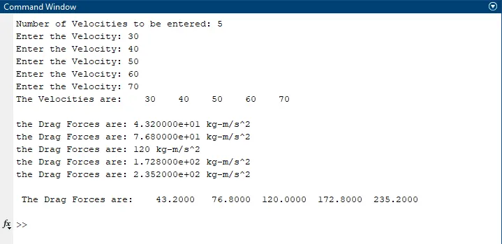
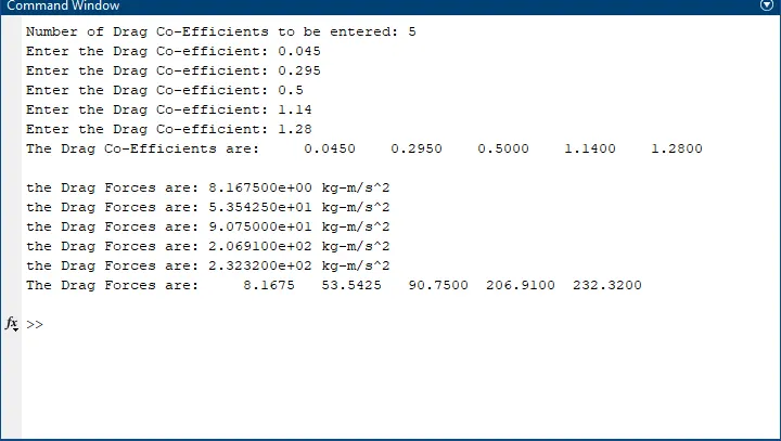
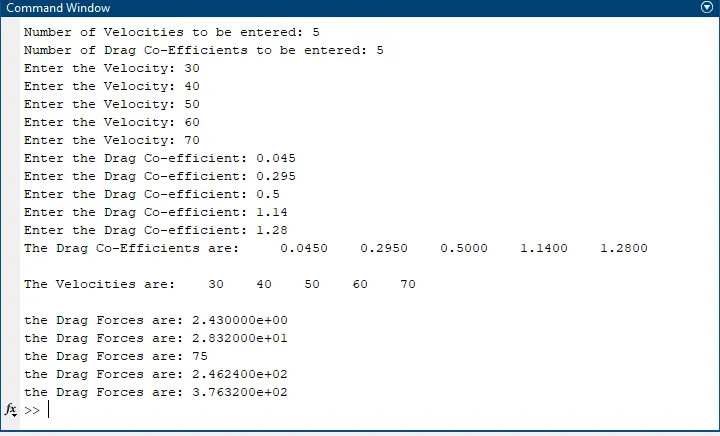
The drag force is calculated and the Values are given below.
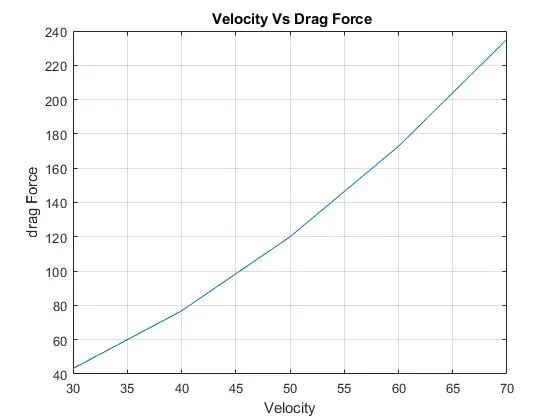
- Velocity Vs Drag Force:
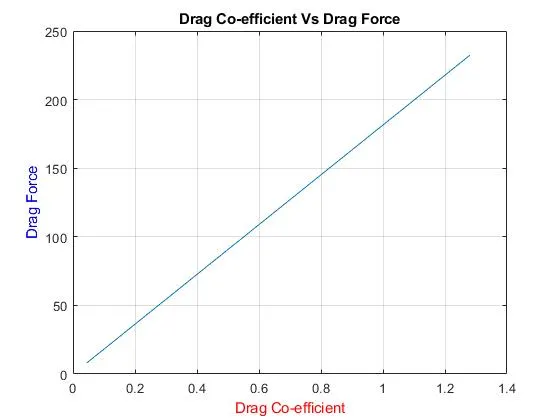
- Drag Coefficient Vs Drag Force:
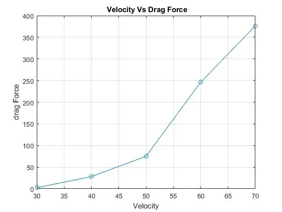
- Different Velocities with Different Drag Coefficient Vs Drag Force:
Graph:
The plot between the Velocity vs Drag Force and the Drag Co-efficient Vs Drag Force is shown.
- Velocity Vs Drag Force:
- Drag Coefficient Vs Drag Force:
- Different Velocities with Different Drag Coefficient Vs Drag Force:
Errors Faced:
The Main error faced while running with different Velocities with different Drag Coefficients is that if the array is of different lengths, the code shows an error 'Matrix Dimensions must agree'.
It means that the Matrix dimension should be the same i.e. Velocity and Drag Coefficients. It can either give the same number of inputs or a row vector.
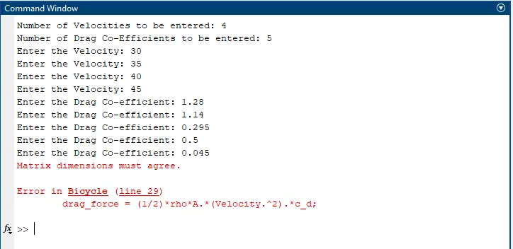
The reason for this error is to give the array the same number of inputs to provide the output. More details are provided in the search bar by clicking the 'Matrix Multiplication'.
Link:
The Research done to get an idea of the Drag force is within the links below.
https://www.simscale.com/blog/2017/07/bike-aerodynamics/
https://en.wikipedia.org/wiki/Drag_coefficient
https://www.sciencedirect.com/science/article/pii/S0167610518305762