Developing MATLAB code for doing stability analysis of linear systems in iterative methods

Aim-: Stability analysis of linear systems in iterative methods

Theory

Basic Iterative Methods :

Iterative methods adopt a completely different approach to the solution of the set of linear algebraic equations. Instead of solving the original equation. A solution vector is initially assumed and through a series of operations the solution vector is systematically corrected towards the solution. Once the error is within acceptable limits, the iterations are stopped. To make the iterative process stable, a preconditioner step (similar to pivoting) can be applied to the system of equations.

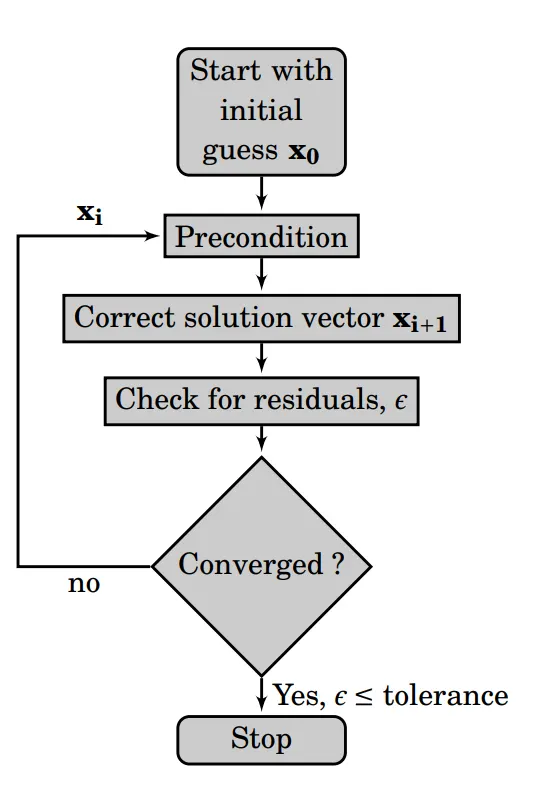
Iterative Methods:

Jacobi

Consider the linear system Ax = b. We may write the coefficient matrix as A = L+D+U where L is strict lower triangular , D is diagonal and U is strict upper triangular . These are respectively given by the following, for a 7×7 matrix (as an example):

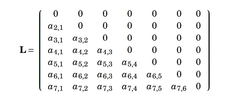
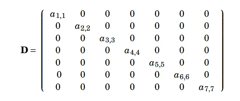
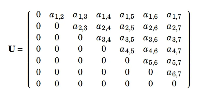
N.B-: 1. Strict lower triangular matrix has non-zero elements for j < i, zero elements for i ≥ j
2. Strict upper triangular matrix has non-zero elements for j > i, zero elements for i ≤ j

We then rewrite the given equation set as

`Dx = b−(L+U)x`

We then write the solution in the form

`x = D ^(−1) [b−(L+U)x]`

This way of writing the equation makes it possible to obtain the solution by an iterativeprocess where a guess value`x^k` is used on the right hand side to obtain an improved value `x^(k+1)` as

`x ^(k+1) = D ^(−1) [b−(L+U)x ^k ]`--------(1)

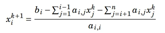
Noting that `D^-1` is also diagonal with elements represented by `1/a_i` the above may be rewritten in the more familiar form

------------(2)

This constitutes what is known as the Jacobi iteration scheme.11 Iteration stops when the change `|x _ i ^(k+1)− x _ i^k | ≤ ε` for 1 ≤ i ≤ n where ε is a prescribed small number.

Gauss Seidel methods

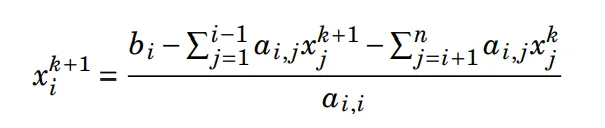
A variant of the above is the Gauss Seidel12 scheme which recognizes that `x_j^(k+1)`for i < j are available during the iteration process and writes the equation set as

--------------(3)

The above may be rewritten in the more familiar form

-------------(4)

successive over-relaxation (SOR)

Another variant is the method of successive under/over-relaxation that is constructed by writing the update as a weighted sum of the old and new values. Thus we would replace Equation (4) by

where ω is known as the relaxation parameter. ω < 1 indicates underrelaxation, ω = 1 represents Gauss Seidel iteration and ω > 1 represents overrelaxation. This may be written in the more convenient form

N.B-: If the coefficient matrix is diagonal dominant, the above methods will converge. In the case of successive over-relaxation method ω < 2.

Using the above mentioned iterative formulas, linear equations has been solved that asked in challenge using MATLAB.

Given condition

Coefficient Matrix, A=[5 1 2 ; -3 9 4; 1 2 -7]

Solution Matrix, X=[x1;x2;x3]

Residual Matrix, B=[10 ;-14; 33]

MATLAB CODE

Functions

Jacobi

function [itr_jac,x_jac] = jac_soln(I_jac,C_jac,x_old)
itr_jac = 0;
err = 10;
residual = 1e-4;
while err>residual
    itr_jac = itr_jac+1;
    x_jac = I_jac*x_old + C_jac;
    err = max(abs(x_jac-x_old));
    x_old = x_jac;
end
end

Gauss-Seidel

function [itr_gau,x_gau] = gau_soln(I_gau,C_gau,x_old)
itr_gau = 0;
err = 10;
residual = 1e-4;
while err>residual
    itr_gau = itr_gau+1;
    x_gau = I_gau*x_old + C_gau;
    err = max(abs(x_gau-x_old));
    x_old = x_gau;
end
end

SOR

function [itr_sor,x_sor] = sor_soln(I_sor,C_sor,x_old)
itr_sor = 0;
err = 10;
residual = 1e-4;
while err>residual
    itr_sor = itr_sor+1;
    x_sor = I_sor*x_old + C_sor;
    err = max(abs(x_sor-x_old));
    x_old = x_sor;
end
end

Main Code

close all
clear all
clc
% coefficient matrix
A = [5 1 2; -3 9 4; 1 2 -7];

n = length(A);

% RHS
B = [10;-14;33];
X = inv(A)*B;
%Eigen values of matrix
a = trace(A);
% Finding sum of minor of digonal element
b = 0;
for i = 1:n
    m=A;
    m(i,: )= [];
    m(:, i) = [];
    d = det(m);
    b = b+d;
end
c = det(A);

% Eqn : x^3 - ax^2 + bx - c = 0
eqn = [1 -a b -c];
% Eigen values of coefficient matrix
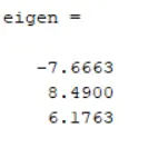
eigen = roots(eqn)
sprectal = max(eigen)


%----------------- ITERATIVE METHODS ---------------%



% matrix decomposition
% Digonal matrix
D_old = zeros(n,n);
for i = 1:n
    D_old(i,i) = A(i,i);
end
% upper triangular matrix
U = zeros(n,n);
for i = 1:n
    for j = 1:n
        if j>i
            U(i,j)=A(i,j);
        else
            U(i,j)= 0;
        end
    end
end

% Lower triangular matrix
L = zeros(n,n);
for i =1:n
    for j= 1:n
        if j<i
            L(i,j) = A(i,j);
        else
            L(i,j) = 0;
        end
    end
end
I = eye(3);


E = 0.5:0.1:1.5;

% effect of changing the diagonal element
for i = 1:length(E)
D = E(i)*D_old;

% Iteration matrix and spectral radius
%Jacobi Method
I_jac = -inv(D)*(L+U);
C_jac = inv(D)*B;
spe_jac(i) = max(abs(eig(I_jac)))

%Gauss_siedel_method
I_gau = -(inv(D+L))*U;
C_gau = (inv(D+L))*B;
spe_gau(i) = max(abs(eig(I_gau)))


% SOR method
%w = 2*(1-sqrt(1-(spe_jac(i))^2))/(spe_jac(i)^2);
w = .9;
%I_sor = (inv(D+w*L))*((1-w)*D-(w*U));
I_sor = I-w*(inv(L+D)*U+I);
C_sor = w*inv(L+D)*B;
spe_sor(i) = max(abs(eig(I_sor)))

% solving equation by iterative method
x_old = [0 0 0]';

[itr_jac(i),x_jac] = jac_soln(I_jac,C_jac,x_old);
[itr_gau(i),x_gau] = gau_soln(I_gau,C_gau,x_old);
[itr_sor(i),x_sor] = sor_soln(I_sor,C_sor,x_old);






end

% plotting results
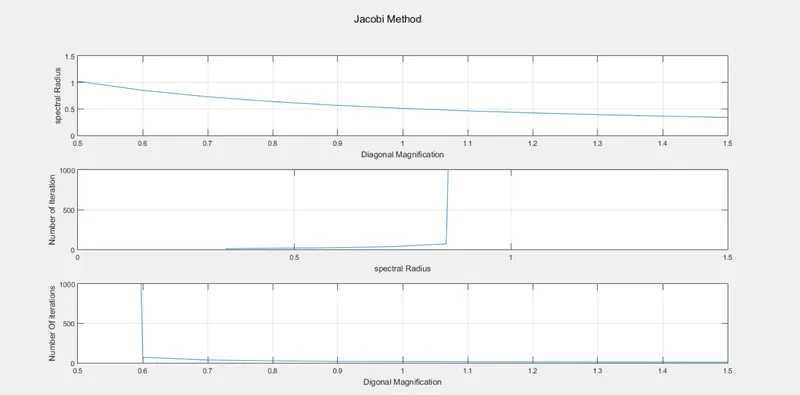
figure(1)
subplot(3,1,1)
plot(E,spe_jac)
xlabel('Diagonal Magnification')
ylabel('spectral Radius')
grid on
subplot(3,1,2)
plot(spe_jac,itr_jac)
xlabel('spectral Radius')
ylabel('Number of Iteration')
axis([0 1.5 0 1000]) 
grid on
subplot(3,1,3)
plot(E,itr_jac)
xlabel('Digonal Magnification')
ylabel('Number Of iterations')
axis([min(E) max(E) 0 1000]) 
grid on
suptitle('Jacobi Method')


figure(2)
subplot(3,1,1)
plot(E,spe_gau)
xlabel('Diagonal Magnification')
ylabel('spectral Radius')
grid on
subplot(3,1,2)
plot(spe_gau,itr_gau)
xlabel('spectral Radius')
ylabel('Number of Iteration')
axis([0 1.5 0 1000]) 
grid on
subplot(3,1,3)
plot(E,itr_gau)
xlabel('Digonal Magnification')
ylabel('Number Of iterations')
axis([min(E) max(E) 0 1000]) 
grid on
suptitle('Gauss-Seidel Method')


figure(3)
subplot(3,1,1)
plot(E,spe_sor)
xlabel('Diagonal Magnification')
ylabel('spectral Radius')
grid on
subplot(3,1,2)
plot(spe_sor,itr_sor)
xlabel('spectral Radius')
ylabel('Number of Iteration')
axis([0 1.5 0 1000]) 
grid on
subplot(3,1,3)
plot(E,itr_sor)
xlabel('Digonal Magnification')
ylabel('Number Of iterations')
axis([min(E) max(E) 0 1000]) 
grid on
suptitle('SOR Method')

Output

PLOT

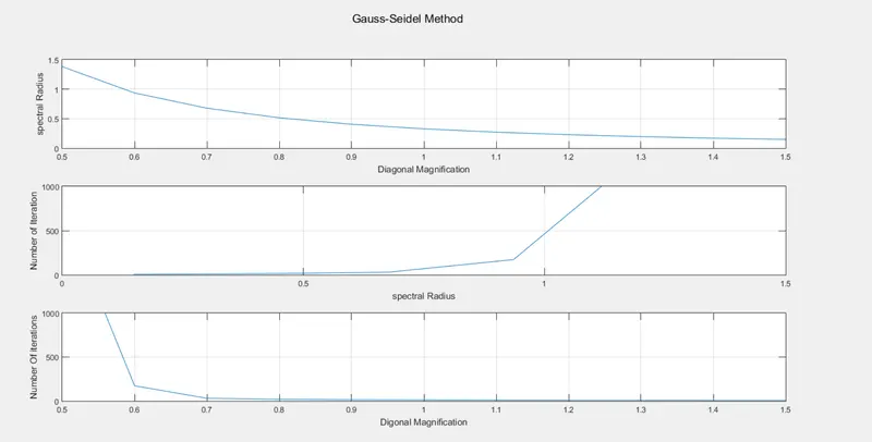
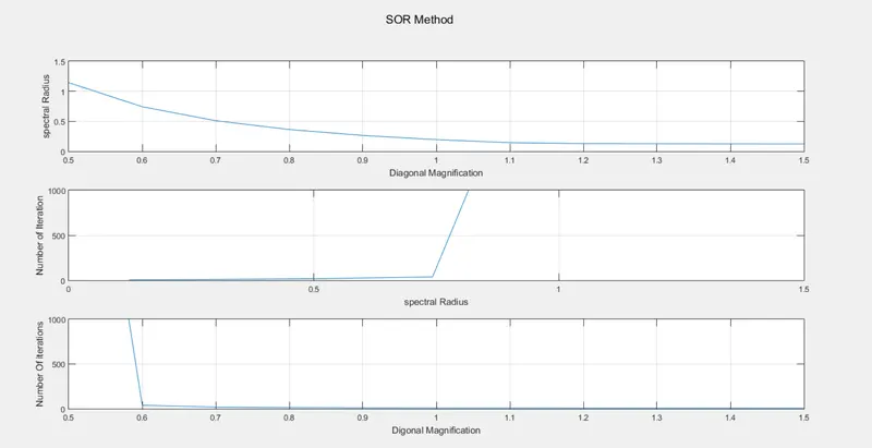
Observation and conclusion

1. If the spectral radius of iterative matrixis less than unity, then error tends to 0 as iteration tends to infinity leading to a converged solution.

2. The rate at which the error decreases is governed, for large iteration number, by the largest eigenvalue of iterative matrix, i.e., by its spectral radius.

3. Thus, the average convergence factor (per step for "m" steps) depends on the spectral radius; the smaller the spectral radius, the larger the convergence factor and the faster the rate of convergence.

4. The asymptotic rate of convergence is proportional to logarithmically. This means that as m tends to ∞, the error decreases by a factor of e for every `1/(− ln [q(P)])` number of iterations, or by one order (factor of ten) for every `2.3/(− ln [rho(P)])` number of iterations. where `rho(p)` is spectral radius of iterative matrix.

5. It can be seen that for such matrices, the SOR method would converge provided the overrelaxation factor satisfied the relation `0<=omega<=2/(1+rho(P)`

6. where `rho(p)` is the spectral radius of the iteration matrix of the pure Jacobi or Gauss-Seidel method (i.e., without overrelaxation). The convergence rate for these methods will depend strongly on the overrelaxation factor and is greatly improved near the optimal relaxation factor, `omega_(opt`, which corresponds to the minimum spectral radius of the iteration matrix.

9. The above results on the conditions for convergence and the rate of convergence expressed in terms of the spectral radius of the iteration matrix are not very useful in practice because of the large size of matrices involved, typically of the order of `10^4xx10^4` or more. The evaluation of the eigenvalues and the spectral radius for such cases may not be practically feasible.

10. A sufficient condition for convergence of an iterative scheme is that the matrix is irreducible and must have general diagonal dominance, i.e.,

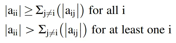
12. It can be seen that under such conditions, the spectral radius of the iteration matrices corresponding to the Jacobi and Gauss-Seidel methods is less than unity and that the two
methods converge for all initial vectors . Also, the SOR method would converge for `0 < omega < 2`.