DESIGN CALCULATIONS OF BAJA SAE ATV

1. Introduction:

In this report a detailed design calculations for the design of BAJA SAE ATV is made. The calculation include design of brake system, suspension system, power train design, steering system design. The requirement for the design is that, the ATV is designed to take part in an competition. To be at a winning position all the theoretical aspect of the ATV should be sound. To achieve best configuration of the ATV a detailed design study and calculations are mandatory. This report explains all the factors affecting the performance of the ATV.

2. Brake system:

2.1.Introduction to Braking System:

The aim of the braking system is to provide a reliable and easy to operate system capable of locking the wheels, and provide continuous control over vehicle’s speed in all terrain. The braking system consists of following components:

2.2. Master Cylinder:

It is a device comprising of two chambers, one chamber is the reservoir containing Brake fluid, which is the working fluid in the braking system and is responsible for compensating any fluid curtail in the brake lines or due to leakage, though rubber seals are used for preventing leakages. The other chamber of the master cylinder is the compression chamber, responsible for retaining pressure in the brake lines even when the brakes are released. As the pedal is pressed, the plunger connected to the pedal moves in opposing the piston return spring’s force to push the piston inside, creating a pressure in the fluid by pressing the fluid present inside the brake line. Eventually creating high pressure inside the calipers leading to compression of brake pads with very high force.

2.3. Brake Calipers:

It is an assembly consisting of brake pads and pistons. Basically there are two types of calipers floating type and fixed type. In the Baja vehicle a fixed type brake caliper is used. A fluid inlet allows high pressure brake fluid to flow inside, creating a pressure inside the cylinder pushing the piston and the brake pads attached to it, eventually creating a high compression force pressing the brake pads against the rotor resulting in decreasing its speed or to stop the rotor.

2.4. Brake Rotor:

The brake rotor also known as the brake disc has an integral function of retarding of the wheel, by applying the braking torque on the wheel. Disc brakes are widely used in the industry as they are better than drum brakes in heat dissipation and cooling down. The rotor is clamped in between the brake pads and they tolerate the compressive forces, from the caliper. The major parameter that decides the size of the rotor is the size of the rim. In the current BAJA buggy as assumed for the discussion, the rims used are of 10 inch diameter, hence, after considering the clearances and mountings of the caliper, it was concluded that the diameter of the rotor to be made would be of 6 inches. The material of the rotor selected is EN – 34 due to its high corrosion resistivity and optimum heat dissipation.

2.5. Brake Pedal:

The brake and accelerator pedal are so designed and placed according to the spaces available after the respective clearances. The pedals should be placed in a way that the driver should not face any hindrance in pressing them with full comfort. The master cylinder should be placed such that it is well protected inside the roll cage. The length of the brake pedal is decided according to the required ratio. A significant consideration while deciding the length of the pedal is the compact nature of the buggy, the area around the pedal is less, which is also covered by the steering column and the steering rack which is shielded hence consuming more space. Therefore, the pedal should have an appropriate length according to the ratio required and should be mounted for unhindered swinging.

2.6. Brake design calculations:

The brake calculations are required to find the minimum distance at which the vehicle will halt on the application of the brake force on the brake pedal. It is necessary to find these values because it gives overall understanding on how to choose the braking systems, like brake cylinders, Brake pedal and other parts. As this ATV is a part of a competition, we need to make sure that highest level of optimisation is done to the vehicle so our vehicle will win in the competition. These calculations will help us achieve our target in terms of weight reduction of the ATV, cost reduction and many other factors.

As per baja rulebook a safe distance should my maintained between the vehicles. At the time of the race braking plays an important role for this condition to be met.

Minimum distance required to stop the ATV:

Input data :

The following are the input data to find the distance of stopping when the brake is applied.

• Mass of the ATV including Driver = 270 kg
• Maximum speed of the ATV = 16.7 m/s
• efficient of friction between ATV and road, µ = 0.7

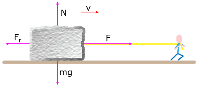
With reference to above image velocity v = 16.7 m/s,

Mass m = 270 kg

Hence, Normal force N = 270 x 9.81 = 2648.7 N

Friction Force, Fr = µ x N

= 0.7 x 2648.7

= 1854.09 N

We need to find Deceleration in order to find the minimum distance.

F = m x a ,

Where F = frictional force (N),

a = deceleration (m²/s)

Hence a = 1854.09/270 = 6.867 m²/s

Using equations of motion,

v² – u² = 2 x a x s,

Where, v = final velocity,

u = initial velocity,

a = acceleration ( in our case deceleration),

s = distance covered.

In order to stop the vehicle the final velocity will be 0

u = 16.7 m/s,

v = 0 m/s,

a = - 6.867 m²/s.

0² = 16.7² + 2x(-6.867)x s

Hence s = 13.78 = 14 m

Therefore the vehicle needs a distance of 14 meters to come to halt at the highest speed possible.

Considering brake forces,

Now we will be calculation the stopping distance based on the pre-defined pedal force. The pedal force of 300 N is applied in order to find the stopping distance.

Pedal Ratio:

Pedal ratio is mechanical advantage given by the distance travelled by the pedal when the force is applied over the pedal. This increases the force given on the master cylinder piston based on a factor, which we call it as pedal ratio. We are considering a pedal ratio of 6.

Force on the master cylinder piston F_mc = F_p x pedal ratio

= 300 x 6

= 1800 N

Pressure applied over the master cylinder piston = F_mc/A_bore

= 22929936 Pa

Static load Calculation

F_f + F_r = mg

We know that moments about the CG is zero.

F_f x W_b = m x g x d

F_f = 2114.66 N

F_r = 1515.03 N

Dynamic load calculation:

DF_f = F_f + (h x mg)/w_b

= 2114.66 + (0.2319 x 3629.7)/1.752

= 2595.1179 N

DF_f mass = 2595.11/9.8 = 264.80 kg

Retardation:

Let the brake for front caliper be 2000 N

F_bf = (DF_f mass x Re )/2

Hence Re = 2000 x 2 /264.80 = 15.105 m / s²

Using equations of motion,

v² – u² = 2 x a x s,

Where, v = final velocity,

u = initial velocity,

a = acceleration ( in our case deceleration),

s = distance covered.

In order to stop the vehicle the final velocity will be 0

u = 16.7 m/s,

v = 0 m/s,

a = - 15.105 m²/s.

0² = 16.7² + 2x(-15.105)x s

Hence s = 9.23 m

Therefore a distance of 9.23m is required when brake is applied with a pedal force of 300 N.

3. Steering calculations:

3.1 Steering Column:

• The steering column is required to control the direction of movement of the Cart.
• The steering Column is designed by following Ackermann steering mechanism.
• The system has a rack and pinion gear set up, tie rod, Heim joint, universal joints, steering wheel for the construction.

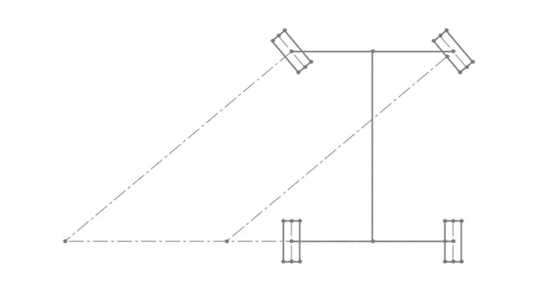
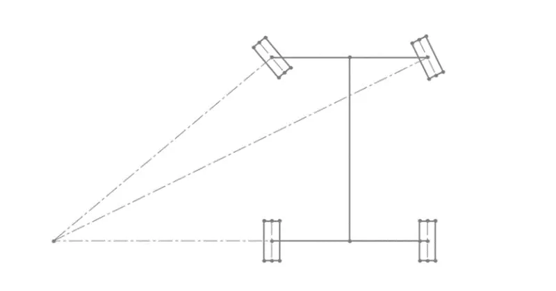
A vehicle with four wheels requires a special steering setup to drive efficiently. If a vehicle were to drive with what is known as parallel steering, at least one tire will scrub along the ground. This is because during a turn, the four tires are not turning about a common point. Instead, three tires are rolling along the ground, while one is slipping. To prevent this, the Ackermann steering setup was invented. Ackermann steering adjusts the steering of each front wheel such that the inside wheel (inside of the turn) is turned more than the outside wheel. For a vehicle with a given wheelbase (𝑙) and front track (𝑤), the outside wheel turn (𝛿_o) for a given inside wheel turn (𝛿_i), or vice versa, can be found using the following equation:

cot 𝛿_o − cot 𝛿_i = 𝑤/l *x

This equation is known as the Ackermann condition. If a given set of the four parameters satisfies the equation with 𝑥=1, that particular set qualifies as 100% Ackermann. However, no simple mechanical linkage configurations can follow the Ackermann condition perfectly throughout the steering motion, so Ackermann is usually stated as the value 𝑥 that satisfies the equation for a particular set of wheel turn angles.

Traction is an important factor in order to manoeuver a vehicle Ackermann steering geometry provide pure rolling motion or prevent slipping of tires, which is appropriate for Baja where there is speed limit of 60 kmph. Whereas anti-Ackermann (reverse ackermann) geometry is used in high speed vehicles, which is appropriate for formula one cars.

Perfect Ackermann steering geometry states that the imaginary line from the steering pivot points inward so as to lie on a line drawn between the steering kingpins and the center of the rear axle. the inner wheel deflects more angle than outer wheel.

3.2. Design Calculation:

Predefined parameters:

1. Base Length = 60” (b)
2. Track Width = 56” (a)
3. Pivot to pivot = 43.7” (c)

Ackermann Angle = Tan^-1(c/2b)

= Tan^-1(43.7/(2*60))

= 20^o

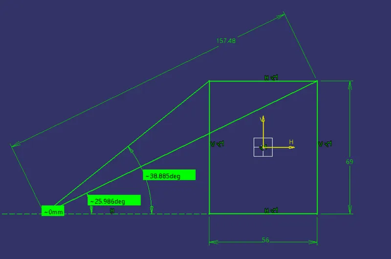
Assuming the turning Radius to be 4mm,

Outer turning angle = 25.986^o = 26^o

By Ackermann equation, cot α – cot β = c/b;

Solving the above equation we get β = 39^o

Where and β are the outer and inner turning angles.

Inner Turning Radius = 2800mm

3.3. Rack and Pinion Design:

Minimum number of tooth in pinion:

Zp = 2h_a / (m*sin²φ)

= 2/(sin²20^o)

= 18

Where,

m = module,

h_a = addendum,

h_f = dedendum,

c = clearance,

Pinion Specifications,

m = 2mm,

addendum = 1*m = 2 mm,

dedendum = 1.25*m = 2.5mm,

clearance = 0.25*m = 0.5mm,

working depth = 2.25*m = 4.5 mm,

tooth thickness = 1.5708*m = 3.14 mm.

m= pcd/ Zp

therefore, pcd = m* Zp = 2 *18 = 36 mm.

where pcd = pitch circle diameter, Zp = number of teeth in pinion.

Steering Ratio:

Approximating maximum turn to be of 25 degrees and steering wheel movement to be 180 degrees the steering ratio can be calculated as,

S.R = 180/25

= 7.2

Rack Travel:

The steer wheel travel for one complete rotation = 2*pi*r

= 691.1 mm

S.R = Steer wheel Travel / Rack Travel.

7.2 = 691.1/rack travel

Rack travel = 95.98 mm = 96 mm.

No. of teeth in the rack:

mp = mr

36/18 = dr/tr

Rack travel = pi*dr

96 = pi*dr

dr = 30.55

= 31

Therefore the number of teeth in rack = 16

4. Power train calculations and design

4.1. Power train:

The powertrain acts as a power plant for the vehicle. Its main purpose is to provide the driving torque at the wheels. This applied torque at the driven wheels causes’ vehicle to move. The power source should be chosen such that it should be able to provide high torque at low rpm and peak power at high rpm. For such dynamic requirement, a stock four cycles, air cooled engine would serve the purpose. This segment has considered Briggs & Stratton (B&S) 10 HP OHV Engine as a prime mover/Powertrain

4.2. Transmission:

The main objective of the transmission is providing to the driver more than the enough torque to the wheels from engine to the wheels. The enough torque means required to pull the driving wheels against the road loads. Road loads include rolling resistance (RR) resistance / air resistance (AR) and grade (GR).To choose the transmission capable of producing enough torque to propel the Baja vehicle, it is necessary to determine the total tractive effort (TTE) requirement of the vehicle. Let us assume an imaginary v following specifications and model.

4.3. Total tractive effort:

The vehicle performance is mainly dependent on two variables: Engine power and Maximum adhesive force between the road and tires (i.e. µ* load on the driving wheels, TE Max). The maximum pull is required when the vehicle is moving uphill at a certain gradient. The gradiability of the vehicle is decided by the amount of torque driving wheels can transmit with maximum allowable tractive effort (TE Max). wheels have such a torque applied to them that they are on the point of slipping in the plane of the wheel, then the value of adhesive force between tire and road surface been reached (µ*WR), where µ adhesion between tire and road weight on the rear wheels. Under these conditions the engine torque has reached the maximum useful value for the present set of conditions, as any increase result in slip and lower acceleration. Static friction is higher than kinetic friction. Total Tractive Effort (TTE) = RR+AR+GR It is suggested to carry out all the calculations on Microsoft Excel for different inclinations and vehicle speed. Such set of data will provide the crystal clear requirement of TTE and the ability of a vehicle to climb without slipping. The TTE corresponding to maximum inclination will be taken as maximum torque which can be applied on wheels by Drivetrain.

Tractive effort = drag resistance + rolling resistance + gradeability

4.3.1. Drag resistance:

A moving vehicle, in displacing the surrounding air has a resultant resisting force called aerodynamic drag or simply air resistance. It can be expressed as resistive force opposing the motion of a vehicle through the air and the work done in overcoming the force is dissipated as energy lost to the air flow.

Drag resistance = r x A x c_d x v² = 68.08 N

where density of air, r = 1.225 kg/m³

cross section area of vehicle = 1 m²

Cd, Coefficient of drag = 0.4

V, Speed of vehicle = 16.67 m/s

4.3.2. Rolling Resistance, Rr (N):

Rolling Resistance (RR) is the force necessary to propel a vehicle over a particular surface. The worst possible surface type to be encountered by the should be factored into the equation.

Rolling resistance = fr x m x g = 115.3124 N

fr, Coefficient of rolling resistance = 0.0435

m, mass of vehicle = 270 kg

4.3.3. Gradeability:

Grade Resistance (GR) is the amount of force necessary to move a vehicle up a slope or “grade”. This calculation must be made using the maximum angle or grade the vehicle will be expected to climb in normal operation.

To convert incline angle, α, to grade resistance:

GR = mg x sin(α)

Where: GR = grade resistance, Newton

mg = gross vehicle weight, Newton

α = incline angle, Degrees

GR= 2648.7*sin(35) = 1364.18 N

Trative effort , Ft(N) = Drag + rolling + grade resistance =1547.575 N

4.4. Minimum required torque (T)

Minimum required torque = Ft x rd = 412.7383 Nm

Where dynamic radius of the wheels rd = 0.2667 m.

4.5. Transmission selection:

The types of transmissions which are very popular among the BAJA teams are: Manual Transmission and Continuous Variable Transmission (CVT). Manual transmission commonly known as gear box can be easily installed and coupled to engine. Use of manual transmission is easy and reliable. The top two best suited gear boxes are Mahindra Alpha and Tata Ace. One of the biggest disadvantages of manual gear box is the ride comfort. The driver comfort is compromise and the fatigue is one of the bad results of using manual gearbox. To increase the comfortability of the driver which will leads to increase in vehicle performance, it is recommended to use CVT which will not only provide the infinite gear ratios between the low and high gear but also helps in reducing the weight and driver fatigue. Therefore in this segment CVT will b discussed However, based on the overall low and high gear ratio calculated in previous segment, one can select the type of gear box required followed by the design of final drive ratio which will be discussed later.

4.5.1. Continuous Variable Transmission (CVT):

The continuous variable transmission (CVT) is plays a most important part in the performance of the vehicle. As stated above, the CVT helps in reducing the driver fatigue as there will be no clutch to press, no lever to shift while changing the gear ration. Thus, it not only save the weight of other components but also provide the smooth ride by allowing driver to shift the infinite number of reductions between the low gear and high gear. Low gear is same as the first gear and high gear corresponds to fourth gear of gear box. The selection of CVT is also due to the fact that the shift in speed and acceleration is continuous with CVT which is in step with gear box. The CVT also allow the engine to run at peak power which is very much desirable for the better performance of the vehicle and good fuel economy of the engine.

4.5.2. CVT selection:

There are many manufactures of CVT like Polaris, Yamaha, Comet, CVTech etc. One can choose from any one of them depending upon the cost, ease of tuning and drive ratios available. Selection of belt is also an important parameter as it is the belt which will be transferring the power. More or less, the belt material same in case of all cvt. On the basis of cost and ease of tuning, it is recommended to use CVTech AAB cvt. CVTech CVT comes with the sponsorship for the BAJA vehicle and is easily available worldwide. The driving ratio of AAB CVT is 6.976, whereas the centre to centre distance of the belt can be selected as per the space. Minimum c/c is 200mm

As mention above, the CVT has low gear and high gear as a fixed ratio CVTech CVT comes with the low ratio of 3 and high ratio of 0.43. According to the need CVT has to be tuned such that shifting occurs at the peak power of the engine and engagement occurs before the peak torque of the engine for the smooth gradual start. Overall reduction required by transmission in low gear was 30. Low ratio of CVT is 3.

Therefore, final drive ratio should be ig_final = 30/3 = 10. This final drive ratio is fixed all the time and normally comprised of larger first gear of gear box differential reduction. But in case of CVT low gear ratio is comparably small and reduction of 10 from CVT to differential is not attainable, hence intermediate reduction is required such that: CVT output shaft is coupled to an intermediate shaft of reduction 2.5. At the end of this intermediate shaft, rest the sprocket which drives the sprocket of differential by reduction of 4. The net final reduction thus comes out to be 2.5*4 = 10 (as required). Therefore net reduction between CVT and Differential is now in two stages. From CVT to differential via intermediate shaft. This arrangement not only saves the space but also pack the entire Drivetrain assembly in smaller area so that the net cg of Drivetrain will lie on the centre line of the vehicle which is very much required

4.5.3. CVT Tuning:

From the previous calculations, it is clear that high gear require to attain the top speed is 0.74 whereas default top gear of CVT is 0.43. That means we need to customize the CVT according to this ratio. This “customization” is nothing but what we called as “CVT TUNING”. Before proceeding for the tuning, one should know the detailed working of CVT. There is no rocket science behind the working of CVT rather a primary (Driving) clutch and a secondary (Driven) clutch connected via belt. The primary clutch has pretension springs and fly weights which control the engagement and shift speed of the system. The secondary clutch is a simple design doing a complicated job. The spring and cam is the key to its performance. Before one starts working on the CVT, two things should be finalized in mind:

1. The ratio required from the CVT at two extreme engine speeds i.e. according to the maximum torque and power.
2. The basic leverage of CVT should not be compromise i.e. CVT should be shifted only at peak power of the engine, allowing the engine to run at its best rated condition. From these two considerations, two graphs should be plotted corresponding to each. In this segment, as engine maximum torque is at 2600rpm, therefore at this instance, CVT should be in low gear. And at 3800rpm, it should be at high gear.

To find the transmission ratio, we use the following formula,

Tractive Effort (Ft) = Te x Tr x nall / rdyn

Hence Tr, transmission ratio = 35

where Te, maximum engine torque = 19.1 Nm

Hence the gear box reduction ratio is chosen as 10:1

4.6. Gear box and gear strength calculations :

Gear material for gear is selected as 20MnCr5 because of its high tensile and yield strength along with appreciable hardness.

Ultimate tensile strength Sut = 1000-1300 N/(mm^2)

Yield Strength Syt = 700 – 900 N/(mm^2)

Hardness = 750 BHN

Stage	No	no of teeth	PCD	module
I	1	18	54	3
I	2	45	135	3
II	3	18	54	3
II	4	72	216	3

First stage design:

No. of teeth in pinion = 18

No. of teeth in gear = 45

Idle speed of the engine = 1750 rpm

Speed available at the pinion = 1750 /3.83 = 456 rpm

Working stress Sbp = Sut/3 = 1100/3 = 366.7 N/(mm^2)

Lewis form factor (Y) = 0.484 – (2.87/Z)

Yp = 0.484 – (2.87/18) = 0.3246

Yg = 0.484 – (2.87/45) = 0.4202

Since Spb x Yp < Sbg x Yg

As pinion is weaker than gear it is necessary to design for the pinion.

Pinion 1: (stage I)

Diameter of pinion (dp) = 54 mm

Face width = 10m = 30 mm

Ratio factor(Q) = (2*Zg)/(Zg+Zp) = (2*45)/(45+18) = 1.429

Load Stress Factor(K) = 0.16*(BHN/100)^2 = 0.16*((650/100)^2)

= 6.76 N/(mm^2)

Beam Strength Fb = Sbp x b x m x Yb = 366.66 * 30*3*6.76

= 1187.978 N

Wear strength Fw = dp x b x Q x K

= 18m x 10m x 1.463 x 6.76

= 16021.61 N

Theoritical Torque calculation:

Maximum available torque from engine = 19.1 Nm

Gear ratio : 10:1

CVT ratio : 0.76 – 3.83

Maximum available torque at wheel shaft = 19.1 x 10 x 3.83

= 731.53 Nm

Minimum available torque at wheel shaft = 19.1 x 10 x 0.76

= 145.16 Nm

As Fb<Fw, Gear Pair is weak in bending hence it is designed for safety against bending.

Maximum available torque at pinion 1 = 19.1 x 3.83 = 73.153 Nm

pitch line velocity at pinion 1 V1 = pi x dp x Np /(60000)

= 3.14 x 18 x 3 x 456 /(60000)

= 1.288656 m/s.

Tangential Force at tooth(Ft) = 2 x T1/dp1

= 2 x 73.153/0.054

= 2709.37 N

Velocity Factor Kv = 6/(6+ V1) = 6/(6 + 1.29) = 0.823045

Service factor(km) = 1.3

Feff = (Km x Ft)/Kv = (1.3 x 2709.37)/0.823045 = 4279.451 N

Let FOS be 2

Feff1 = Fw/fos = 16021.6/2 = 8010.8 N

since Feff < Feff1 our design is good to go

Second Stage :

Torque in second stage pinion shaft = 182.8825 Nm

Number of teeth in pinion Zp = 18

Number of teeth in gear Zg = 72

Speed of Pinion Np = 456/2.5 = 182.4 m/s

Gear ratio = 4

Sbp = Sut/3 = 1100/3 = 367 N

Lewis form factor Yp = 0.484 - (2.87/Zp) =0.324555556

Yg = 0.484 - (2.87/Zg) = 0.444138889

Pinion is weaker than gear.

Diameter of pinion = 54 mm

Face Width(b) = 30 mm

Ratio Factor (Q) = 2xZg/(Zg+Zp) =1.6

Load Stress Factor (K) N/mm^2 = 0.16 x (BHN/100)^2

= 0.16x(650/100)^2

= 6.76

Beam Strength Fb = Sbp x b x m x Yp = 366.66 x 30 x3x0.324

= 10709.96 N

Wear Strength (Fw) = dp x b x Q x K = 54 x 30 x 1.6 x 6.76

= 17521.92 N

As Fb< Fw, Gear Pair is weak in bending hence it is designed for safety against bending

Torque at pinion 2 = 182.8825

Pitch line velocity at pinion 2 V2 m/s = pi x dp x Np/(60 x 1000)

= 3.14 x 54 x 182/(60000)

= 0.514332 m/s

Tangential Force at tooth (Ft) = 2 x T2/dp

= 2 x 183/0.054

= 6777.778 N

Velocity Factor (Kv) = 6/(6+V2) =6/(6+0.514332) = 0.921046

Service Factor (Km) = 1.3

Feff = (km x Ft)/ Kv = (1.3+6777)/0.921046

= 7359.35 N

Checking Gear pair for wear strength

Fw = FOS x Feff

FOS = 17521.92/7359.35 = 2.34

Since FOS is above 2 the design is good to go.

5.Suspension System:

The suspension system is responsible to make the driver comfort while driving. The suspension system is responsible for isolating the road vibrations and forces created while riding in bad road conditions and bumpy roads. The design of suspension is very important for a vehicle.

Spring Dimensions:

Height of the spring (uncompressed) = 177 mm

Compressing length = 100

5.1. Spring Stiffness Calculation

F = kx , where F = force or load applied over the spring

k = spring stiffness,

x = compression length

Dynamic load in the front side of ATV = 2114.6627 N

For each spring Load = 2114.6627 /2

= 1057.3 N

K1= 1297.6/0.100 = 10573 N/m

Dynamic load in the rear side of ATV = 1515.0373 N

For each spring Load = 1515.0373 /2

= 757.52 N

K2 = 1297.6/0.100 = 7575.2 N/m

5.2. Spring diameter calculation:

X = 8F(D^3) n/ (G(d^4))

Where, F = load applied on the spring

D = Spring coil diameter

d = spring wire diameter

G = modulus of rigidity (material property)

n = number of coils.

Considering few constants for the calculation of coil diameter,

Let the wire diameter be 10 mm,

Number of turn or coils = 12

Modulus of rigidity = 79.3 GPa ( High carbon spring wire)

X = 8F(D^3) n/ (G(d^4))

Therefore D = 68.40 mm

6. Conclusion:

The design considerations and calculation are done for the ATV and the 3D model for the done calculation is optimised and is ready for further phases.

7. References:

• https://www.irjet.net/archives/V5/i10/IRJET-V5I10325.pdf
• https://www.irjet.net/archives/V7/i2/IRJET-V7I227.pdf
• https://www.ijert.org/research/braking-calculation-for-a-baja-atv-IJERTV10IS040079.pdf
• https://ijaems.com/upload_images/issue_files/1452664386-6%20IJAEMS-JUL-2015-11-Design%20of%20a%20Drivetrain%20for%20Sae%20Baja%20Racing%20Off-Road%20Vehicle.pdf
• https://www.ijert.org/design-and-analysis-of-gearbox-for-sae-baja-competition
• https://www.tribology-abc.com/calculators/properties_of_common_spring_materials.pdf