Cyclone Separator Challenge

Aim: To perform analysis on cyclone separator and calculate the separation efficiency and pressure drop. 

 Introduction of Cyclone separators:

Cyclone separators or simply cyclones are separation devices (dry scrubbers) that use the principle of inertia to remove particulate matter from the flue gases(The gas exiting to the atmosphere via a flue, which is a pipe or channel for conveying exhaust gases from a fireplace, oven, furnace, boiler or steam generator). Cyclone separators is one of many air pollution control devices known as pre-cleaners since they generally remove larger pieces of particulate matter. 

Their simple design, low maintenance costs, and adaptability to a wide range of operating conditions such as sizes and flow rates make cyclones one of the most widely used particle removal devices. This prevents finer filtration methods from having to deal with large, more abrasive particles later on. In addition, several cyclone separators can operate in parallel, and this system is known as a multi-cyclone.

                                   

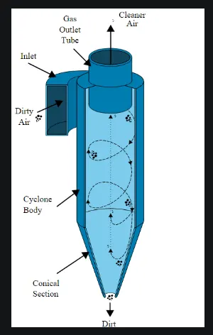
The four empirical models which are used to calculate the cyclone separate efficiency are:

1. IOZIA AND LEITH MODEL

 Iozia and Leith logistic model is a modified version of Barth Model, which is developed based on force balance. The model assumes that a particle carried by the vortex endures the influence of two forces: a centrifugal force, Z, and flow resistance, W. The collection efficiency `eta_i` of particle diameter `d_(p i)` can be calculated from

  `eta_i = 1/(1+(d_(pc)/d_(p i))^beta)`

`beta` = is an expression for the slope parameter

2. LI AND WANG MODEL

 The Li and Wang model include particle bounce or re-entrainment and turbulent diffusion at the cyclone wall. A two-dimensional analytical expression of particle distribution in the cyclone is obtained. Li and Wang model was developed based on the following assumptions:
• The radial particle velocity and the radial concentration profile are not constant for uncollected particles within the cyclone.
• Boundary conditions with the consideration of turbulent diffusion coefficient and particle bounce re-entrainment on the cyclone wall. The tangential velocity is related to the radius of the cyclone.

`eta_i = 1- exp{-lambdatheta_1}`

3. KOCH AND LICHT MODEL

 Koch and Licht collection theory recognized the inherently turbulent nature of cyclones and the distribution of gas residence times within the cyclone. Koch and Licht described particle motion in the entry and collection regions with the additional following assumptions:
• The tangential velocity of a particle is equal to the tangential velocity of the gas flow, i.e. there is no slip in the tangential direction between the particle and the gas.
• The tangential velocity is related to the radius of the cyclone by:  `uR^n` = constant.

A force balance and an equation on the particles collection yields the grade efficiency 

`eta_i = 1-exp{-2[(Gtau_iQ)/D^3(n+1)]^(0.5/(n+1))}`

G is a factor related to the configuration of the cyclone, n is related to the vortex and `tau` is the relaxation term.

4. LAPPLE MODEL

 Lapple model was developed based on force balance without considering the flow resistance. Lapple assumed that a paricle entering the cyclone is evenly distributed across the inlet opening. The particle that travels from inlet half-width to the wall in the cyclone is collected with 50% efficiency. The semiempirical relationship developed by Lapple to calculate a 50% cut diameter, `d_(pc)`.

The efficiency of collection of any size of the particle is given by:

`eta_i = 1/(1+(d_(pc)/d_(p i))^2)`

Geometry:

 Import the geometry file extract the volume.

After the volume extraction: 

                                       

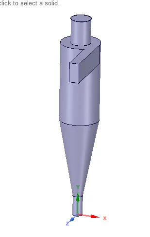
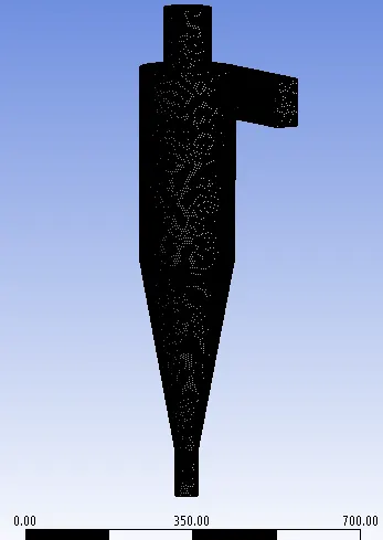
Mesh:

Mesh size: 5mm 

The number of nodes: 584569

Name the faces inlet, outlet_1(the outlet for the lighter air or particles), and outlet_2(the outlet for the heavier particles). 

                                 

Setup:

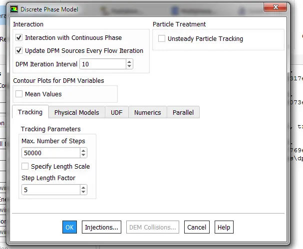
  Open fluent < click on steady time < gravity, y= -9.81 < Models < select K-epsilon < RNG < swirl dominated flow < ok < close. Open discreate phase model < click on interaction with continuous phase and update DPM < click on injections and create the  injection and check on the "inject using face normal direction", with the velocity = 3m/s and diameter = 5`mum` , with the surface as the injection type and inlet to the defined. 

                 

        

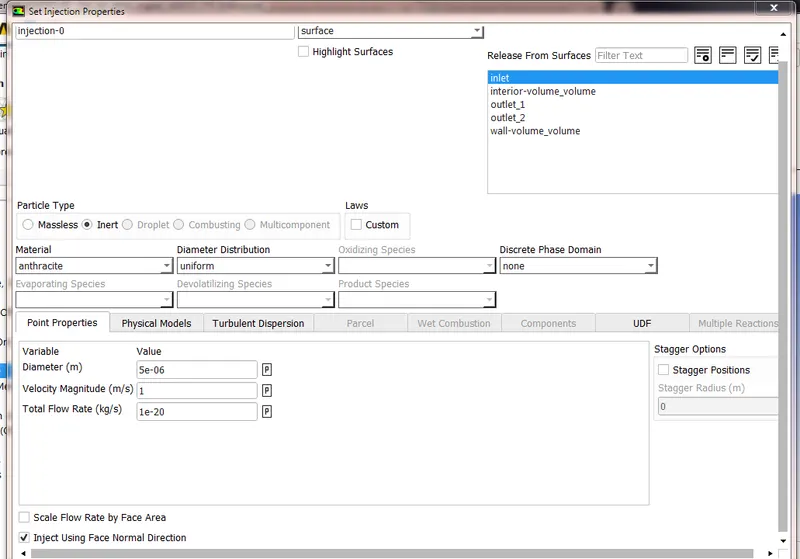
Click on boundary conditions and select the DPM as given in the challenge for inlet, outlet1, and outlet2. Open solutions methods and change second-order upwind for turbulent K.E and turbulent dissipation rate < select standard method < and click on options and compute from the inlet < open residuals and uncheck the convergence criteria column < click on initialize and run the calculation for 600 iterations. After that export the particle history date which was used in the CFD results.   

Case 1: Varying the particle diameter[1`mum`,3`mum`, and 5`mum`] and velocity as 3m/s.

1`mum`:

 

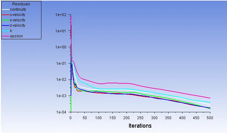
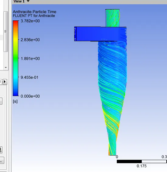
https://www.youtube.com/watch?v=y3Zx_G15m8I&ab_channel=Harsha

 Efficiency = Trapped particles/Total particles 

               =  234/438 = 0.534%   

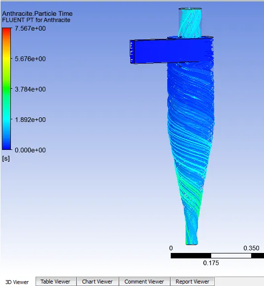
3`mum`:

 

 

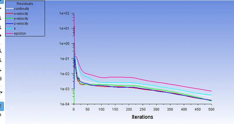
https://www.youtube.com/watch?v=0zHEBLIxOSM&ab_channel=Harsha

 Efficiency = Trapped particles/Total particles 

               =  270/438 = 0.616%

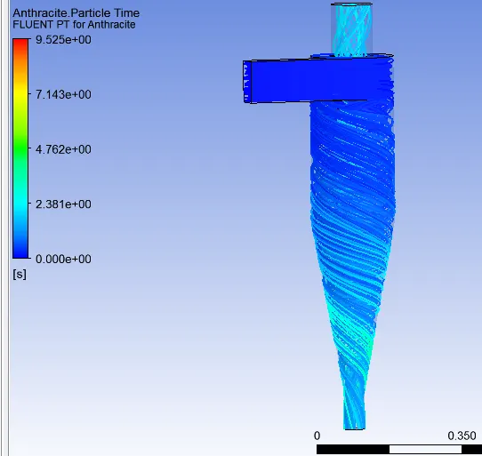
 5`mum` :

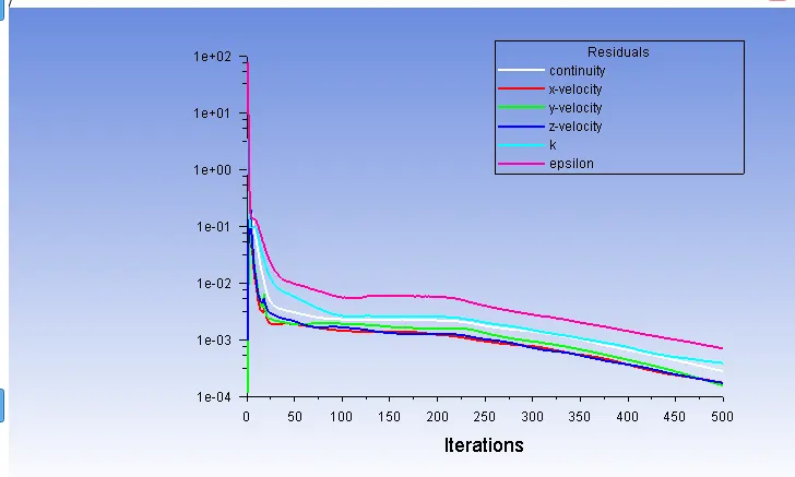
Residuals: 

 

https://www.youtube.com/watch?v=6t6w6Hvzjyk&feature=youtu.be&ab_channel=Harsha

Efficiency = Trapped particles/Total particles 

               =  321/438 = 0.732%

Case 2: Varying the velocity[1m/s, 3m/s, and 5m/s] and particle diameter as 5`mum`.

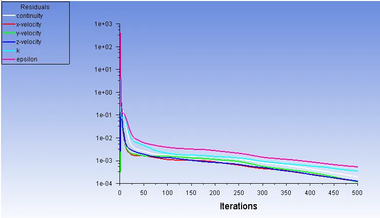
1m/s:

 

 

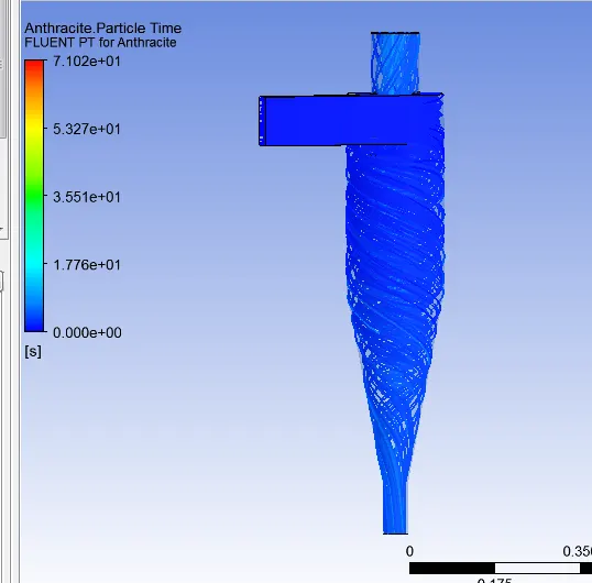
https://www.youtube.com/watch?v=U2nffg_5A4M&ab_channel=Harsha

 Efficiency = Trapped particles/Total particles 

               =  203/438 = 0.463% 

 3m/s:

Residuals: 

 

https://www.youtube.com/watch?v=6t6w6Hvzjyk&feature=youtu.be&ab_channel=Harsha

 Efficiency = Trapped particles/Total particles 

               =  321/438 = 0.732%

5m/s:

Residuals:

 

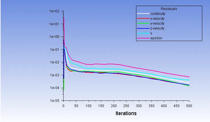
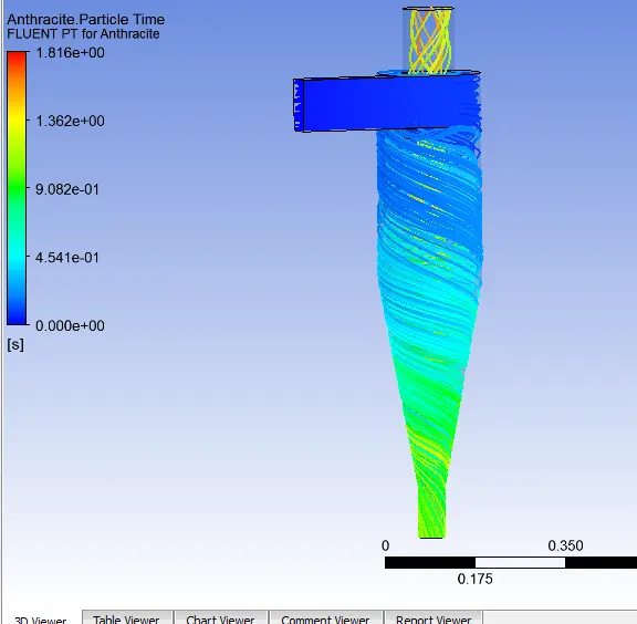
https://www.youtube.com/watch?v=HZb8Omr2_Lw&ab_channel=Harsha

 Efficiency = Trapped particles/Total particles 

               =  369/438 = 0.842% 

S.No	Velocity	Diameter	No. tracked	Escaped	Aborted	Trapped	Evaporated	Incomplete	Incomplete     parallel	Efficiency
1.	3m/s	1`mum`	438	204	0	234	0	0	0	0.534
2.	3m/s	3`mum`	438	167	0	270	0	1	0	0.616
3.	3m/s	5`mum`	438	115	0	321	0	1	1	0.732
4.	1m/s	5`mum`	438	210	0	203	0	25	0	0.463
5.	3m/s	5`mum`	438	115	0	321	0	1	1	0.732
6.	5m/s	5`mum`	438	69	0	369	0	0	0	0.842

Conclusion:

From the above table, the efficiency of a cyclone separator depends on both velocity and particle diameter size. If the velocity and particle diameter size increase then the efficiency also increases. 

Comparing case 1 and case 2, the velocity plays an important role in increasing efficiency. If the velocity increases then the efficiency also increases.