Cyclone Separator Challenge
Aim:- To perform analysis on cyclone separator and calculate the separation efficiency and pressure drop.
Objective:-
- To write a few words about any four empirical models used to calculate the cyclone separator efficiency.
- To perform an analysis on a given cyclone separator model by varying the particle diameter from 1 μm to 5 μm and calculate the separation efficiency in each case. Discuss the results. [Use both the velocity's as 3m/sec.]
- To perform an analysis on a given cyclone separator model by varying the particle velocity from 1 m/sec to 5 m/sec and calculate the separation efficiency and pressure drop in each case. Discuss the results. [Use particle diameter size as 5 μm for all cases & keep flow velocity same as particle velocity]
Introduction:
Cyclone separators are separation devices that use the principle of inertia to remove particulate matter from flue gases. Cyclone separator is one of many air pollution control devices known as pre-cleaners since they generally remove larger pieces of particulate matter. This prevents finer filtration methods from having to deal with large, more abrasive particles later on. In addition, several cyclone separators can operate in parallel, and this system is known as a multi-cyclone.
It is important to note that cyclones can vary drastically in their size. The size of the cyclone depends largely on how much flue gas must be filtered, thus larger operations tend to need larger cyclones. For example, several different models of one cyclone type can exist, and the sizes can range from a relatively small 1.21.5 meters tall (about 4-5 feet) to around 9 meters (30 feet)—which is about as tall as a three-story building.
Removed Components from Cyclone Separators:
Dust Particles: Abrasive, Corrosive, Adhesive, Explosive
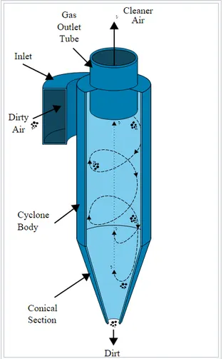
Diagram:
Process Description:
Working Principle:
A cyclone is a centrifugal separator in which particles, due to their mass, are pushed to their outer edges as a result of centrifugal force. Incoming Air is automatically forced to adopt a fast revolving spiral movement – the so-called double vertex. This double spiral movement consists of an outer stream, which flows downwards in a spiral, and an inner stream, which flows upwards in a spiral. At the interchange between both streams, air passes from one stream to another. The particles which are present in the air re forced to the outer edges and leave the separator via a collection device fitted to the bottom of the separator.
The airspeed of the cyclone lies between 10 to 20 m/s, and the most common speed is 16 m/s. If there are fluctuations in speeds (with lower speeds), separation yield falls quite drastically.
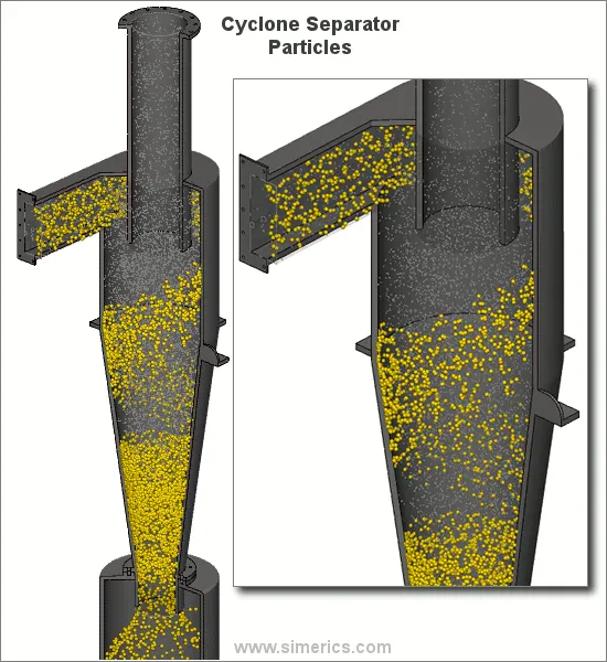
Most cyclones are built to control and remove particulate matter that is larger than 10 micrometers in diameter. However, there do exist high-efficiency cyclones that are designed to be effective on particles as small as 2.5 micrometers. As well, these separators are not effective on extremely large particulate matter. For particulates around 200 micrometers in size, gravity settling chambers or momentum separators are a better option.
Out of all of the particulate-control devices, cyclone separators are among the least expensive. They are often used as a pre-treatment before the flue gas enters more effective pollution control devices. Therefore, cyclone separators can be seen as "rough separators" before the flue gas reaches the filtration stages.
Four common Empirical models for Cyclone Separator Efficiency:
1. Iozia and Leith Model:
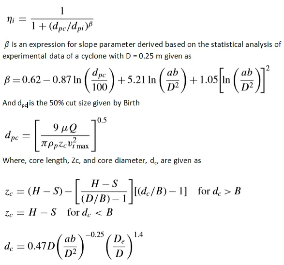
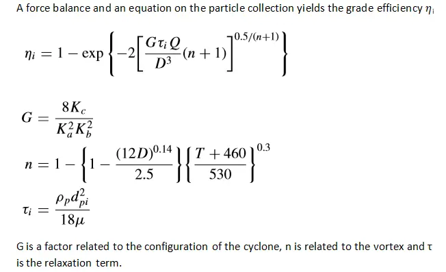
Iozia and Leith logistic Model is a modified version of the Barth (1956) model which is developed based on force balance. The model assumes that a particle carried by the Iozia and Leith logistic Model is a modified version of the Barth (1956) model which is developed based on force balance. The model assumes that a particle carried by the vortex endures the influence of two forces: a centrifugal force Z, and flow resistance, W.
The collection efficiency i of particle diameter dpi can be calculated by,
2. Li and Wang Model:
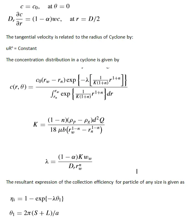
The Li and Wang model include particle bounce or re-entrainment and turbulent diffusion at the cyclone wall. A two-dimensional analytical expression of particle distribution in the cyclone is obtained. Li and Wang's model was developed based on the following assumptions:
The radial particle velocity and the radial concentration profile are not constant, for uncollected particles within the cyclones.
Boundary conditions with the consideration of turbulent diffusion coefficient and particle bounce re-entrainment on the cyclone wall are:
3. Koch and Licht Model:
Koch and Licht collection theory recognized the inherently turbulent nature of cyclones and the distribution of gas residence times within the cyclone.
Koch and Licht describe particle motion in the entry and collection regions with the additional following assumptions:
1. The tangential velocity of a particle is equal to the tangential velocity of the gas flow, i.e. there is no slip in the tangential direction between the particle and the gas.
2. The tangential velocity is related to the radius of cyclone by uRn =constant.
4. Lapple Model:
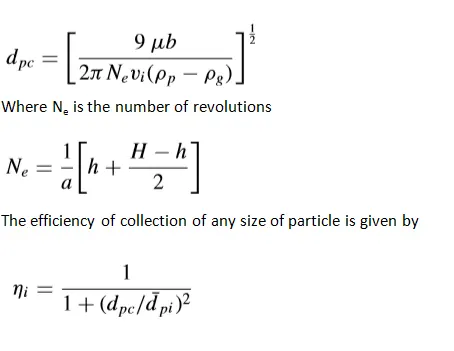
Lapple model was developed based on force balance without considering the flow resistance. Lapple assumed that a particle entering the cyclone is evenly distributed across the inlet opening. The particle that travels from inlet half-width to the wall in the cyclone is collected with 50% efficiency. The semi-empirical relationship developed by Lapple to calculate a 50% cut diameter, dpc, is
Applications:
Chemical and Petrochemical Processes
Industrial, Metallurgical, and Power Generation
Food & Pharmaceutical
Cement Industry
_ _ _ _ _ _ _ _ _ _ _ _ _ _ _ _ _ _ _ _ _ _ _ _ _ _ _ _ _ _ _ _ _ _ _ _ _ _ _ _ _ _ _ _ _ _ _ _ _ _ _ _ _ _ _ _ _ _ _ _ _ _ _ _ _ _ _ _ _ _ _ _ _ _ _ _ _
Methodology:
There are two different Phases as given below:
Continuous Phase
Discrete Phase
Continuous Phase:
It consists of fluid flowing within the fluid volume
Discrete Phase:
It consists of smaller particles interacting with the Continuous Phase.
It can also exchange momentum, mass, and energy with Fluid Phase or Continuous Phase.
To carry out this analysis,
The simulation will be done using DPM (Discrete Phase Modeling).
Discrete Phase Modeling:
It is employed when there are solid Particles in Gas, or Liquid or Liquid Droplets in Gas, or Bubbles in Liquid.
There are two ways to carry out DPM
1. Un-coupled Flow
2. Coupled Flow
Uncoupled Flow:
In this type of flow, the Discrete Phase will not have any interaction with the Continuous Phase.
Coupled Flow:
It will influence the flow of the Continuous Phase.
Since the size of the particles injected into the Cyclone Separator is very small, the usage of both types of flow should not matter much.
Setup and Simulation
In this project, we will perform an analysis of a given Cyclone model in two different manners.
1) By varying particle diameters
2) By varying particle velocities
As per condition, we will discuss theses analysis in two different parts in the following section below:
Geometry:
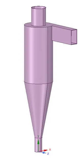
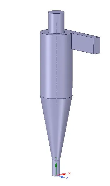
Extract the fluid volume within the geometry by selecting the inner edges at inlet and outlets.
Creation of fluid volume and geometry of Cyclone Separator as given below:
Meshing:
Here the geometry of the Cyclone Separator is simple and so we can create hexahedron elements for the fluid volume. ''Cut cell'' approach is used to generate structural meshing as it gives the best result.
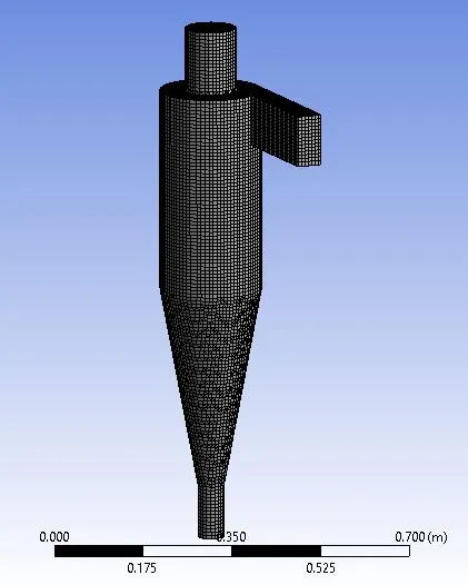
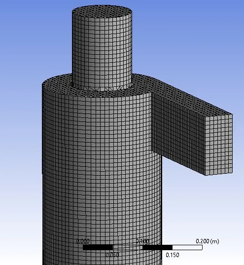
Mesh settings, statistics, and cell arrangements are as given below:
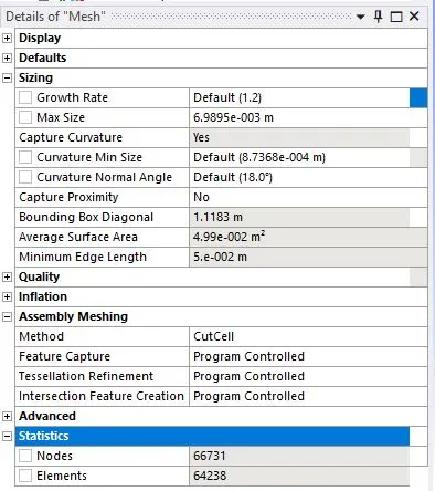
Also, we have to create Named selections for different kinds of behavior at inlet and outlets.
Named selections are as per given below:
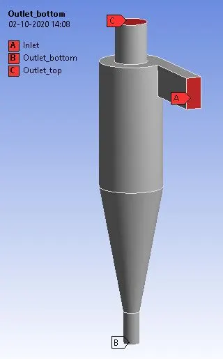
As we can see Inlet, Outlet_Top, Outlet_Bottom, and the rest of that are named as Wall by default by Ansys Fluent.
Here we have given two Outlets purposely.
Outlet_Top is used for light gas and Outlet_bottom is used for collecting heavy particles, which drops due to gravity at the bottom.
Physical and Boundary condition:
After completing Meshing, we further go to the Setup in fluent.
Here we will see the case set up for both Part_1 and Part_2 cases.
Solver Type: Pressure Based
Time: Steady
Gravity: -9.81 m/s2 (in –Y direction)
Viscous Model: > Model: K-Epsilon
> K-Epsilon Model: RNG
> RNG Option: Swirl Dominated Flow
> Near Wall Treatment: Standard Wall Functions
Here RNG is the slight modification of the Standard K-Epsilon model.
This enhances the accuracy of the swirling flows.
DPM Settings:
Here we will see the setting for both Part_1 and Part_2 cases as given below:
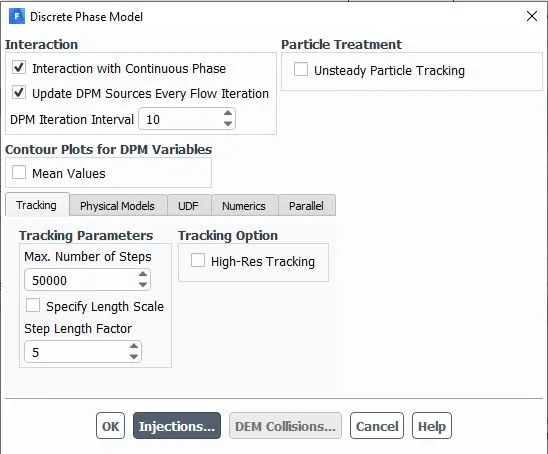
As per the above image, enable the “Interaction with Continuous Phase”. This will enable the Coupled Flow.
Also, enable “Update DPM Sources Every Flow Iteration”. Enabling this option gives the chance to calculate the Particle Source Terms at every Iteration. (For Unsteady Simulation, it is recommended, and given by-default.)
Set “DPM Iteration Interval = 10”. This option allows us to control the frequency at which particles attract.
Here “Tracking Parameters = 50000”. It is the maximum number of Time Steps, to compute a single trajectory of Particle. In case, the fluent exceeds the maximum number of Time Steps, it will automatically cancel the report of Trajectory. For the Steady case,
Time Steps number = 50,000 given by default. But for calculation of all possible particles, we have set it to 1500000.
“Step Length Factor = 5”. This is used to control the size of the Time Step. The larger the Factor, the smaller the Time Step will be.
Here, we have not used the “Specify Length Scale”, which is also used for controlling the Time Step size, by dividing Length Scale with Velocity of Discrete Particle and Velocity with Velocity of Continuous Phase.
Particle Injection:
Particle injections setting for Part_1 and Part_2 cases are as given below:
Here in Injection, select “Create”.
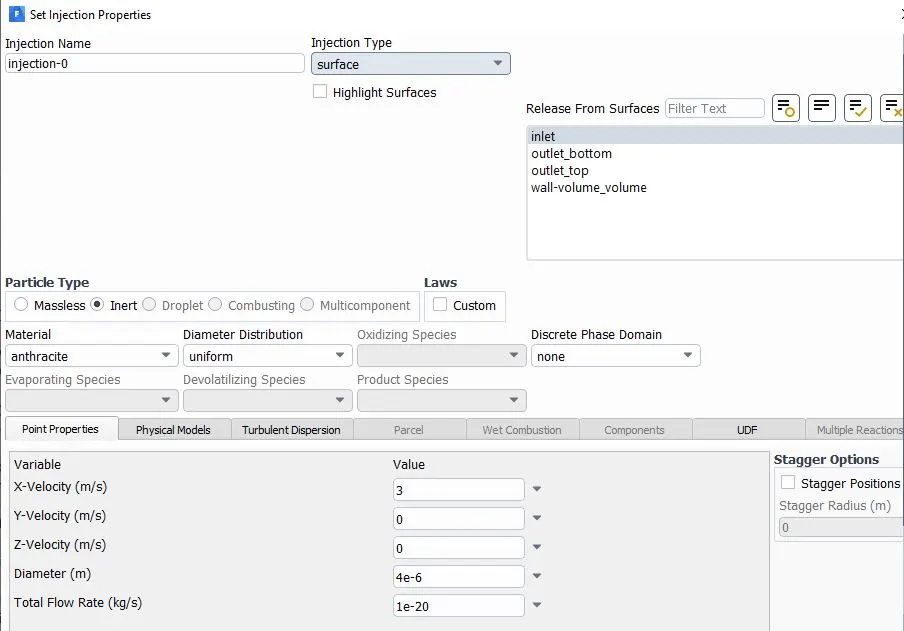
From the above image, give appropriate “Injection name” as per different cases.
Common settings for all cases are as given below:
Injection Type: Surface
Release From Surface: Inlet
Particle Type: Inert
Material: Anthracite
Flow Rate: 1e-20 Kg/s
Boundary Condition:
Inlet and wall:- Reflect
Outlet(Top):- Escape
Outlet(Bottom/dustbin) - Trap
Reflect: It is the Particle Rebound off the boundary in question with a change in its momentum as defined by the coefficient of restitution.
Escape: The particle is reported as having “escaped” when it encounters the boundary in question. Trajectories calculated are terminated.
Trap: The Trajectory calculated is terminated and the fate of the particle is recorded as “trapped”. In the case of the evaporating droplets, their entire mass instantaneously passes into the vapor phase and enters the Cell adjacent to the boundary. in the case of a combusting particle, the remaining volatile mass is passed into the vapor phase.
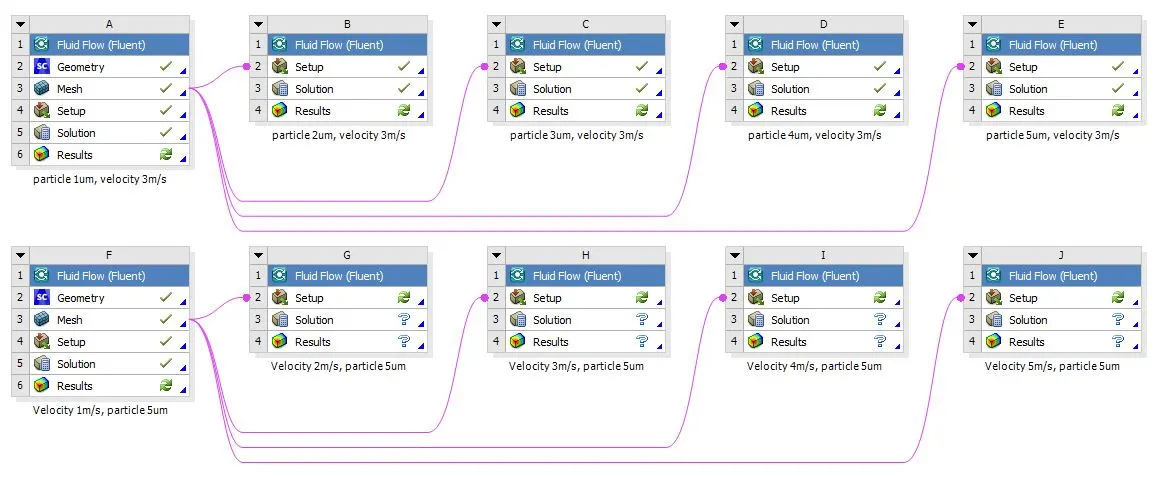
The below image shows the ANSYS Fluent setup of all the simulations for both the cases.
Results:
In this section, we will see the results of all the cases of both parts respectively.
Here we will see the Results of Part_1 and Part_2 and calculate the Separation Efficiency and Pressure Drop for each case.
Separation efficiency:
It is defined as the fraction of particles of a given size collected in the cyclone, compared to those of that size going into the cyclone. Experience shows that the separation efficiency of cyclone separator increases with increasing particle mean diameter and density; increasing gas tangential velocity; decreasing cyclone diameter; increasing cyclone length; extraction of gas along with solids through the cyclone legs.
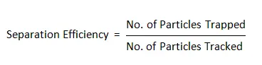
In this case, depending upon the particle history data - Separation Efficiency is defined as the ratio of concentration that has been removed from the feed stream to the initial concentration in the feed stream. For this case ratio of the number of trapped particles to the total number of particles tracked.
Pressure Drop:
The pressure drop across the cyclone is of much importance in a cyclone separator. The pressure drop significantly affects the performance parameters of a cyclone. The total pressure drop in a cyclone will be due to the entry and exit losses, and friction and kinetic energy losses in the cyclone. Normally the most significant pressure drop occurs in the body due to swirl and energy dissipation.
Pressure drop is defined as the difference in total pressure between two points of a fluid carrying network.
Pressure drop = Total inlet pressure - Total Outlet Pressure
As the “escape” DPM condition is given to the outlet-top in this case, so outlet-top is considered in pressure drop calculation.
Case 1.1 (Velocity 3m/s, particle diameter 1 μm) :
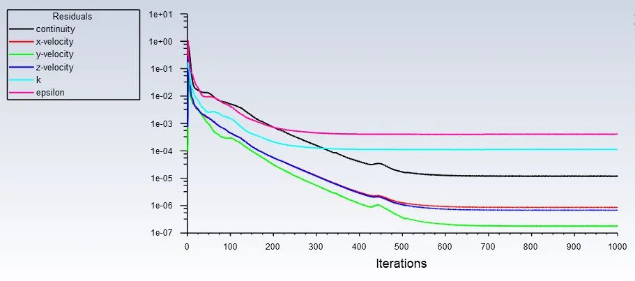
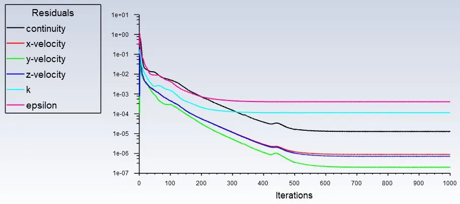
Residuals:
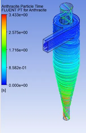
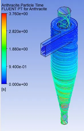
Particle Resident Time:
Particle Tracking:

Separation Efficiency in % = (32 / 98) * 100
Separation Efficiency = 33.06 %
Pressure Contour: Velocity Contour:
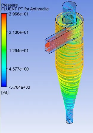
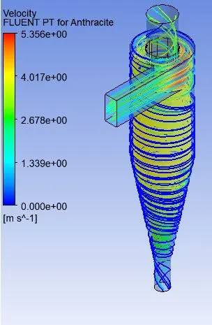
Case 1.2 (Velocity 3m/s, particle diameter 2 μm) :
Residuals:
Particle Resident Time:
Particle Tracking:

Separation Efficiency in % = (64 / 98) * 100
Separation Efficiency = 65.30 %
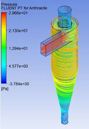
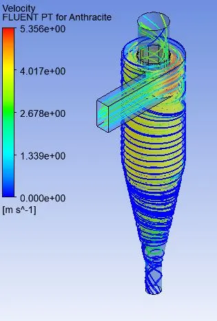
Pressure Contour: Velocity Contour:
Case 1.3 (Velocity 3m/s, particle diameter 3 μm) :
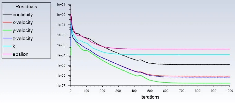
Residuals:
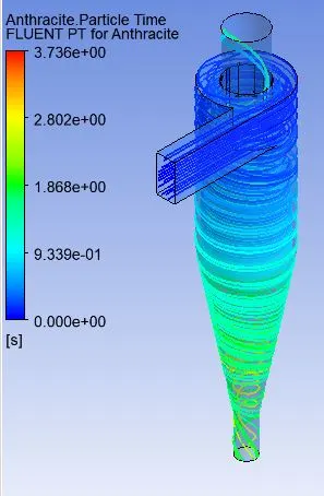
Particle Resident Time:
Particle Tracking:

Separation Efficiency in % = (76 / 98) * 100
Separation Efficiency = 77.55 %
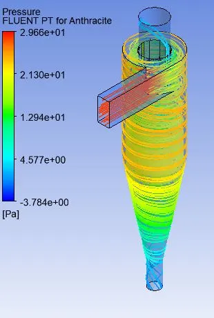
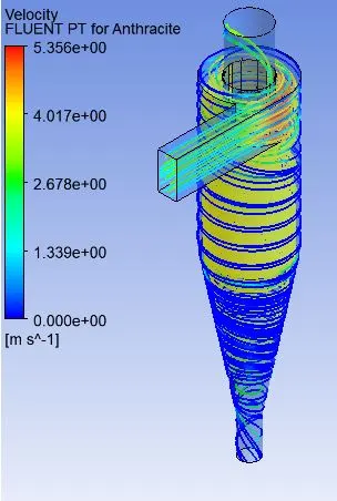
Pressure Contour: Velocity Contour:
Case 1.4 (Velocity 3m/s, particle diameter 4 μm) :
Residuals:
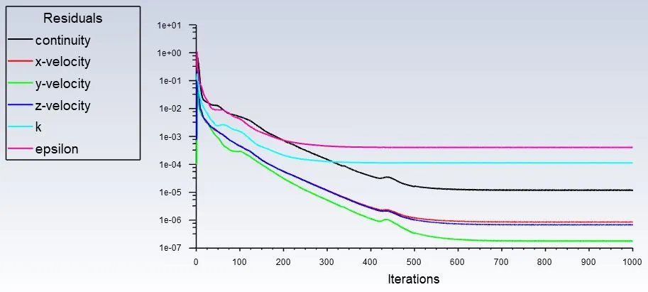
Particle Resident Time:
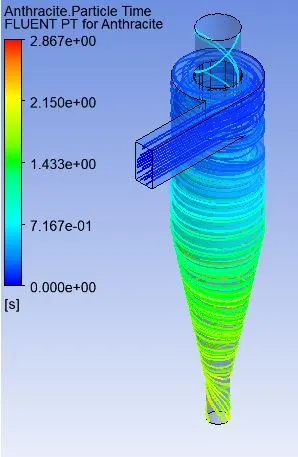
Particle Tracking:

Separation Efficiency in % = (86 / 98) * 100
Separation Efficiency = 87.75 %
Pressure Contour: Velocity Contour:
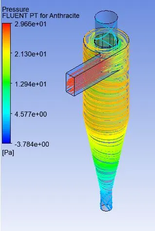
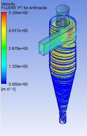
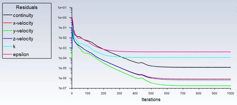
Case 1.5 (Velocity 3m/s, particle diameter 5 μm) :
Residuals:
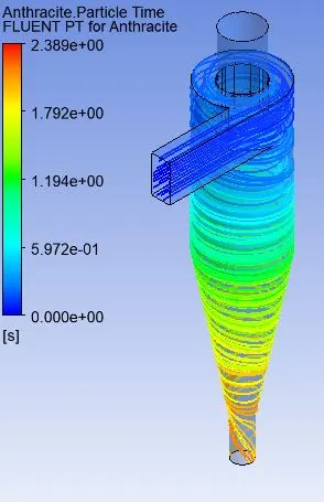
Particle Resident Time:
Particle Tracking:

Separation Efficiency in % = (97 / 98) * 100
Separation Efficiency = 98.97 %
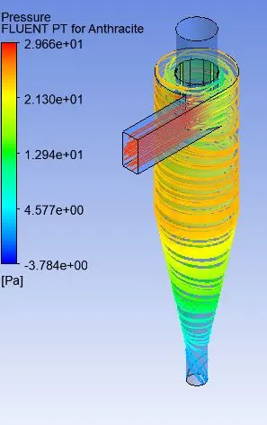
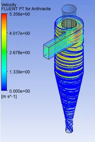
Pressure Contour: Velocity Contour:
_ _ _ _ _ _ _ _ _ _ _ _ _ _ _ _ _ _ _ _ _ _ _ _ _ _ _ _ _ _ _ _ _ _ _ _ _ _ _ _ _ _ _ _ _ _ _ _ _ _ _ _ _ _ _ _ _ _
Results for case 2 with varying particle velocity from 1m/s to 5m/s. :
Case 2.1 (Particle and Flow Velocity 1m/s, particle diameter 5 μm) :
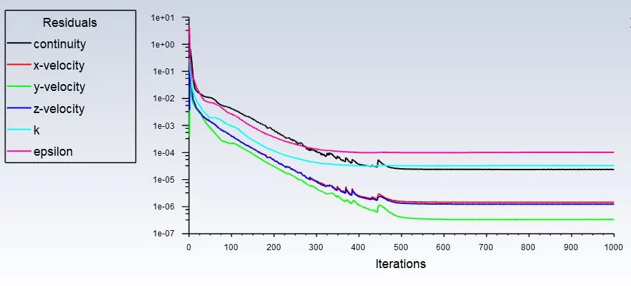
Residuals:
Particle Resident Time:
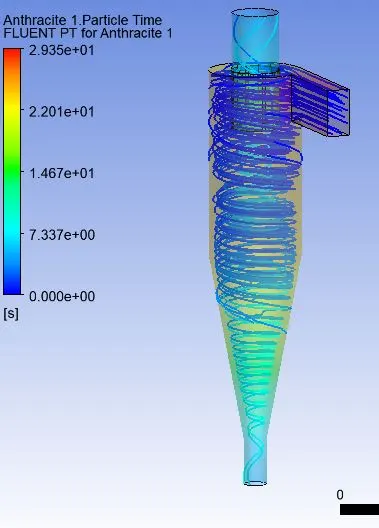
Particle Tracking:

Separation Efficiency in % = (9 / 98) * 100
Separation Efficiency = 9.18 %
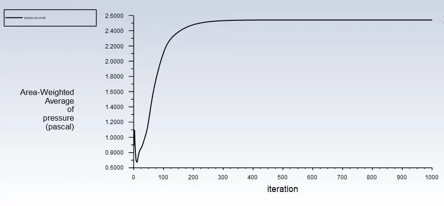
Pressure Drop:
Inlet:
Outlet_Top
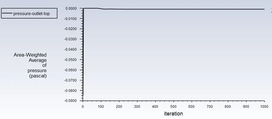
Total Pressure:
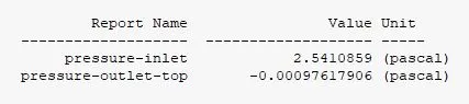
Pressure drop = Total inlet pressure - Total Outlet Pressure
= 2.5410 – (-0.00097)
Pressure drop =2.5420 Pa
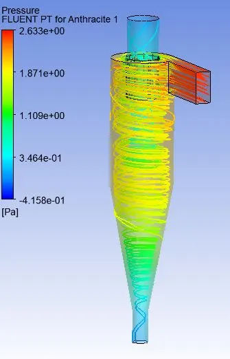
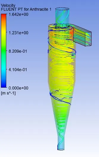
Pressure Contour: Velocity Contour:
Case 2.2 (Particle and Flow Velocity 2m/s, particle diameter 5 μm) :
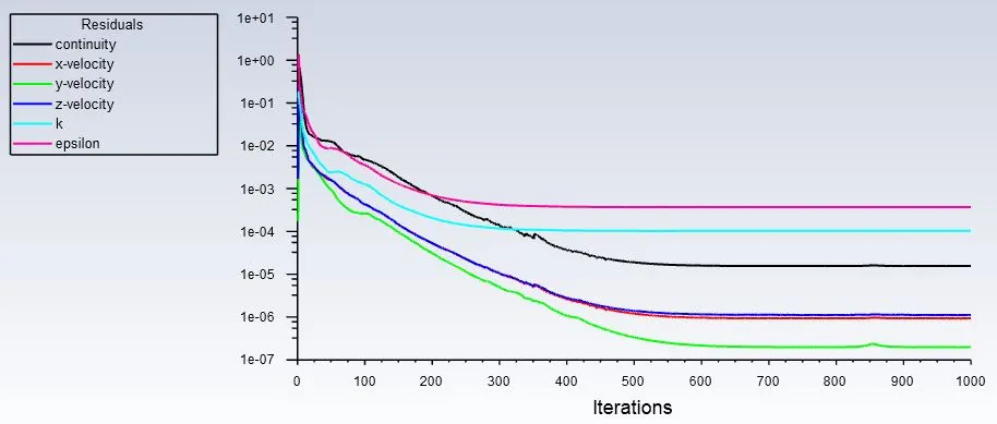
Residuals:
Particle Resident Time:
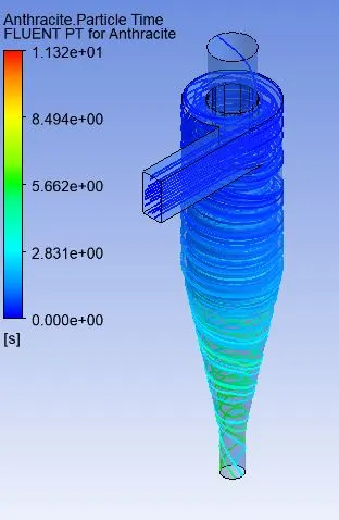
Particle Tracking:

Separation Efficiency in % = (38 / 98) * 100
Separation Efficiency = 38.77 %
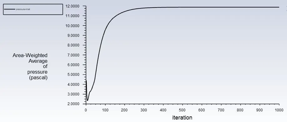
Pressure Drop:
Inlet:
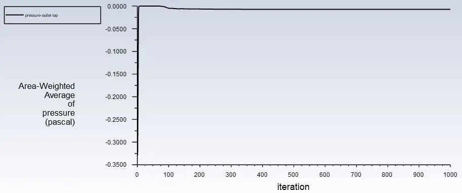
Outlet_Top
Total Pressure:
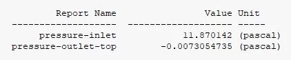
Pressure drop = Total inlet pressure - Total Outlet Pressure
= 11.870142 – (-0.0073054)
Pressure drop = 11.8773 Pa
Pressure Contour: Velocity Contour:
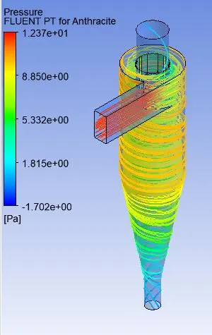
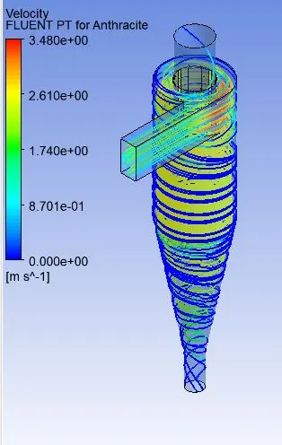
Case 2.3 (Particle and Flow Velocity 3m/s, particle diameter 5 μm) :
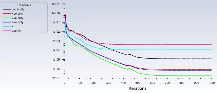
Residuals:
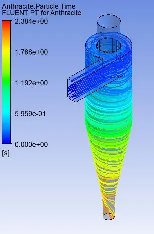
Particle Resident Time:
Particle Tracking:

Separation Efficiency in % = (97 / 98) * 100
Separation Efficiency = 98.97 %
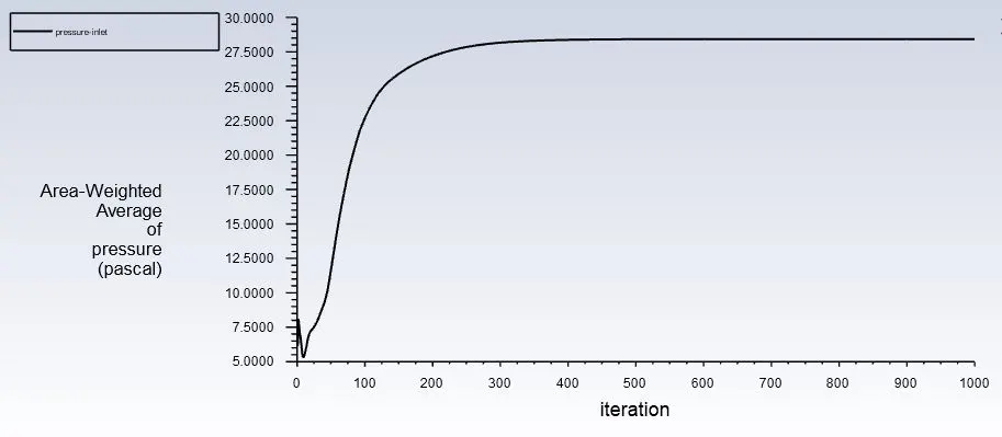
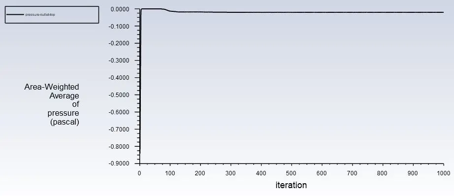
Pressure Drop:
Inlet:
Outlet_Top
Total Pressure:
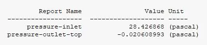
Pressure drop = Total inlet pressure - Total Outlet Pressure
= 28.426868 – (-0.02060899)
Pressure drop =28.447476 Pa
Pressure Contour: Velocity Contour:
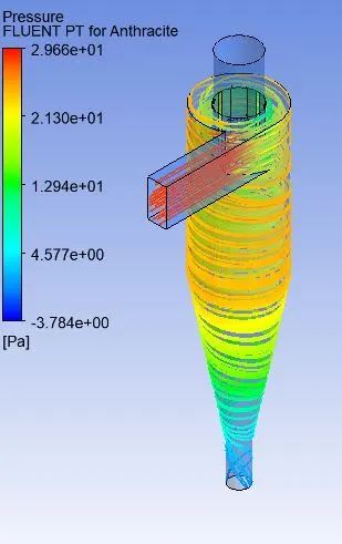
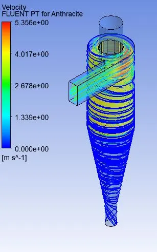
Case 2.4 (Particle and Flow Velocity 4m/s, particle diameter 5 μm) :
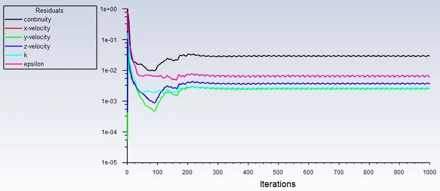
Residuals:
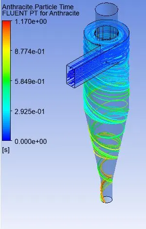
Particle Resident Time:
Particle Tracking:

Separation Efficiency in % = (98 / 98) * 100
Separation Efficiency = 100 %
Pressure Drop:
Inlet:
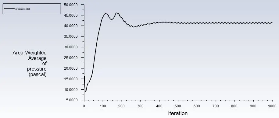
Outlet_Top
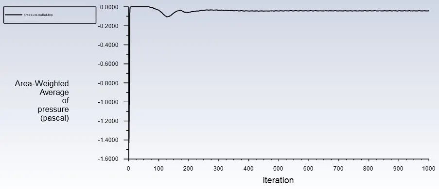
Total Pressure:
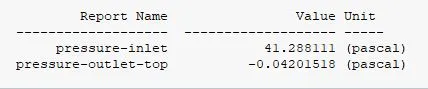
Pressure drop = Total inlet pressure - Total Outlet Pressure
= 41.288111 – (-0.04201518)
Pressure drop = 41.33012618 Pa
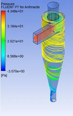
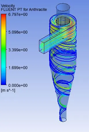
Pressure Contour: Velocity Contour:
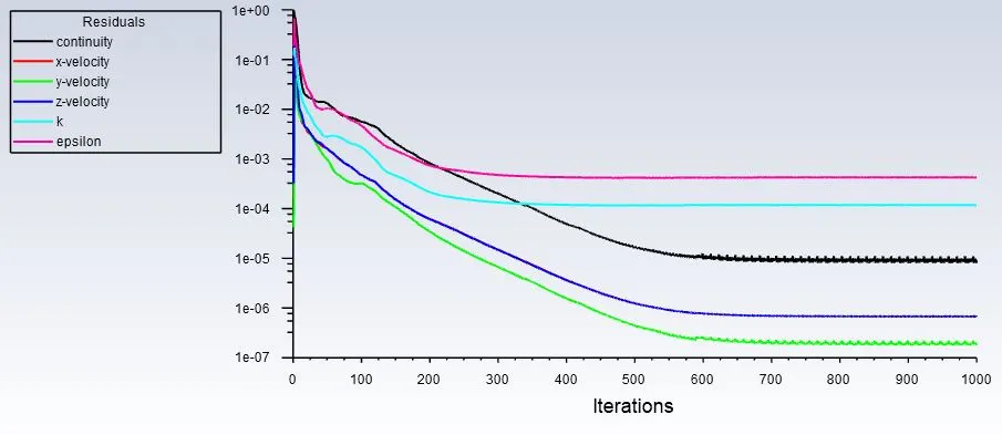
Case 2.5 (Particle and Flow Velocity 5m/s, particle diameter 5 μm) :
Residuals:
Particle Resident Time:
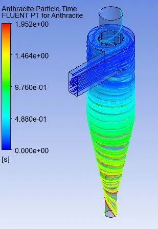
Particle Tracking:
Separation Efficiency in % = (98 / 98) * 100
Separation Efficiency = 100 %
Pressure Drop:
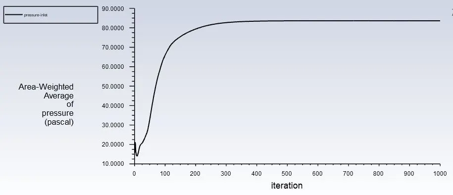
Inlet:
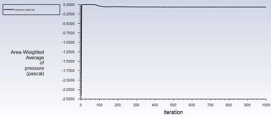
Outlet_Top
Total Pressure:

Pressure drop = Total inlet pressure - Total Outlet Pressure
= 83.631569 - (-0.067713054)
Pressure drop = 83.69928 Pa
Pressure Contour: Velocity Contour:
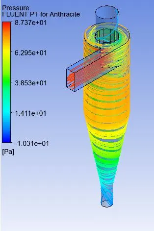
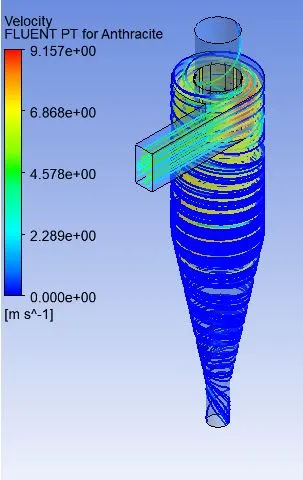
Cyclone efficiency generally increases with the increase in inlet velocity. The efficiency of a cyclone separator is related to the pressure drop across the separator.
COMPARISON TABLE:
Case_1:
|
Size of Particle |
The velocity of the Particle | Particle tracked | Particle Trapped | Separation efficiency | Pressure drop (in Pascal) |
| 1 μm | 3 m/s | 98 | 32 | 32.65 % | 28.44 |
| 2 μm | 3 m/s | 98 | 64 | 65.30 % | 28.44 |
| 3 μm | 3 m/s | 98 | 76 | 77.55 % | 28.44 |
| 4 μm | 3 m/s | 98 | 86 | 87.75 % | 28.44 |
| 5 μm | 3 m/s | 98 | 97 | 98.97 % | 28.44 |
Case_2:
|
Size of Particle |
The velocity of the Particle | Particle tracked | Particle Trapped | Separation efficiency | Pressure drop (in Pascal) |
| 5 μm | 1 m/s | 98 | 9 | 9.18 % | 2.54 |
| 5 μm | 2 m/s | 98 | 38 | 38.77 % | 11.87 |
| 5 μm | 3 m/s | 98 | 97 | 98.97 % | 28.44 |
| 5 μm | 4 m/s | 98 | 98 | 100 % | 41.33 |
| 5 μm | 5 m/s | 98 | 98 | 100 % | 83.69 |
Conclusion:
1. From the observations of both the cases, we can conclude that the Separation efficiency of the Cyclone Separator depends on both Diameter of Particles and also on the Particle Velocity.
2. Also, we can conclude that in the 2nd Case, there are more efficient results. So the Velocity is a more effective variable for higher efficiency.
3. The efficiency of a Cyclone Separator has a direct effect on the Pressure Drop. Higher efficiency Cyclones have the highest Pressure Drops.
5. Higher the Velocity, hence higher the Pressure Drop, and higher the Efficiency.
6. Also we can observe that, with increases in the Diameter of the Particle and Velocity of the Particle, Particle Resident Time decreases. So, when less Resident Time is taken by the Particles, the efficiency of the Cyclone Separator can be high.