CFD Analysis of Airfoils with Rotating Cylinder forWind Turbines
Chapter 1 Introduction
Mankind is harvesting energy from natural resources for centuries. There are a lot of means of generating energy from renewable sources out of which Wind is one of the primary sources. Over the years a number of researches have been conducted to increase the efficiency of Wind turbines by changing its design. Most Modern wind turbines operate on a principle of Airfoil shaped cross-section blades. Irrespective of the method used, the main objective is to delay the boundary Layer flow separation over the blade to generate more lift from the wind turbine [1]. This thesis work based on one such method to use the principle of Magnus the effect, as such, to delay the boundary layer separation on the surface of an airfoil.
1.1 Magnus effect
The Magnus effect is referred to as a generation of lift from spinning cylinders or spheres. The lift force generated by the Magnus effect is much larger than streamlined aerofoils. This has motivated a large number of researchers and scientists to use the Magnus lift in aerospace, naval, and wind turbine industries. Perhaps it was Anton Flettner who has patented using Magnus lift and employed it in his ship Buckau as shown in the image below. [2]
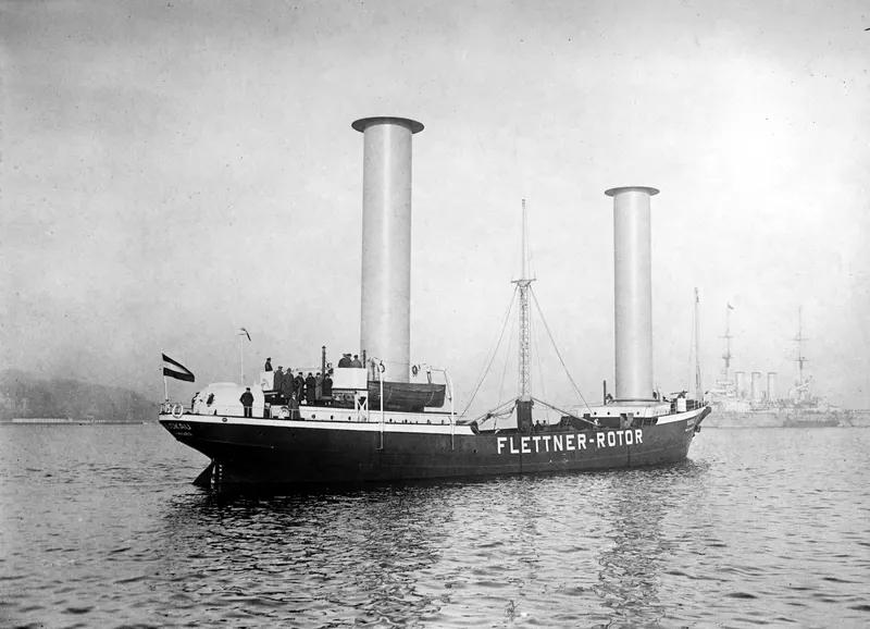
FIGURE 1.1: The Buckau, the first vehicle to be propelled by a Flettner rotor [3]
The Magnus effect is named after Gustav Magnus, the German physicist who investigated it. It describes the force generated by fluid flow over a rotating body, at right angles to both the direction of flow and the axis of rotation. This force on a rotating cylinder is known as Kutta–Joukowski lift, after Martin Kutta and Nikolai Zhukovsky (or Joukowski), who first analyzed the effect. [4]
As can be visualized from the figure below The Magnus effect, depicted with a back-spinning cylinder or ball in an air-stream. The arrow represents the resulting lifting force. The curly flow lines represent a turbulent wake. The airflow has been deflected in the direction of spin.
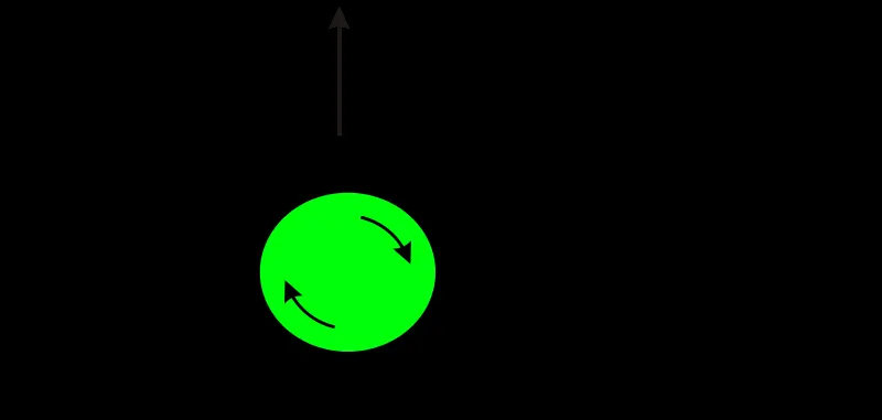
FIGURE 1.2: Magnus effect on Rotating cylinder
"The fluid medium surrounding a spinning rotor may be visualized as concentric circles resembling a section of a sliced onion. The boundary layer nearest the core circulates most rapidly and the speed diminishes with each subsequent ring. As the fluid begins to flow past the cylinder, these concentric layers arranged themselves into streamlines, and as the rotational speed increases those on the side moving in the same direction as the flow converges, indicating diminished pressure. The streamlines on the opposite side, moving against the current, become more widely spaced showing an increase in pressure. This pressure differential manifests itself as a "lifting" force and tends to displace the rotor at a right angle to the fluid flow and in the direction of the side of the rotor that is moving in the same direction as the fluid stream." [5]
1.2 Application of Magnus effect on Wind Turbine Aerodynamics
Modern wind turbines mainly work on the principle of aerodynamics. Wind turbines extract kinetic energy from the wind by aerodynamic forces acting on a blade surface and convert it into mechanical energy. Airfoil section tends to generate lift when the relative wind strikes at the leading edge of the blade section at a certain angle of attack. There are mainly two types of aerodynamic forces of our importance namely lift force and drag force. Lift force acts in a perpendicular direction of a relative wind direction and drag force acts in the direction of the relative wind. The Power extraction and loads on a wind turbine are mainly influenced by these aerodynamic forces. Hence the power output of any wind turbine depends on the interaction between the turbine rotor and wind.
Magnus principle can also be applied to wind turbine applications for the generation of lift and Power production. Over the year different types of concepts and designs are used to run wind turbines based on the Magnus effect. The figure below shows one such Magnus wind turbine.
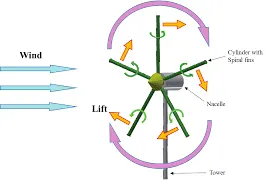
FIGURE 1.3: MagnusWind Turbine [6]
"The lift force generated by the Magnus effect is much larger than streamlined airfoils. The turbine uses a rotating cylinder as a substitution for the blade of the common wind turbine. When the cylinders rotate, the lift is generated. This lift is sufficient to generate electricity by rotating the wind turbine to which the cylinders are attached. The wing of the wind turbine is a column shape, and, in the Magnus wind turbine, the power performance increases from the increase in lift. The Magnus wind turbine currently in operation produces 3 kW electric power at wind speed 8 m and starts at cut-in wind speeds above 4 m/s. The rotation of the cylinder uses about 8% of the electricity generation [6]. However, to accelerate commercialization, it is desirable to improve performance even more." [7]
1.3 Summary of work
The main task of this thesis is to observe the repercussion of the Magnus effect on Wind Turbine. To observe that two different modified designs of an airfoil are used. Rotating cylinders are placed at the Leading and Trailing edge of an airfoil. Symmetric Joukowsky airfoil with 15% thickness is used in this thesis work. By cutting ones leading part and trailing part suitable arrangement of geometry is created to fit the cylinder at the leading and trailing edge respectively.
Modified airfoil geometries are then used for computing aerodynamic forces. Numbers of factors affect the forces data in the airfoil namely rotation of the cylinder, Reynolds number of the flow, the gap between the cylinder and airfoil surfaces, etc. This thesis work focuses on these basic factors which affect the aerodynamic forces.
Several Experimental works over the year are performed on similar types of modified airfoil geometries. Nowadays CFD (Computational Fluid Dynamics) analysis has taken over the conventional form of modeling in modern engineering problems as more and more high performing computational tools are available. This thesis work uses the Ansys Fluent CFD tool to perform a series of simulations over the modified airfoil geometry. After performing several simulations and collecting aerodynamic force data, these data then compare with similar experimental results for its validity.
After the CFD simulation, this thesis work will conclude about the eventuality of the Magnus effect on the modern wind turbine. Also how different modifications on airfoil might leads to interesting changes in the lift and drag force. These changes, if positive and practically possible can be further used in real-life applications to have more efficient wind turbines.
1.4 Computational Fluid dynamics
“Computational fluid dynamics (CFD) consists of solving the differential equations governing fluid flow using approximate numerical means. In principle, with sufficient grid refinement, the solution of the discretized governing equations yields a flow that is a reasonable representation of reality, at least within the context of the underlying assumptions used to derive the model equations (i.e., incompressibility, in stationarity, etc.).” [8]
In earlier days CFD was used for the analysis of two-dimensional airfoils. Nowadays with an increase in power of computing, we can use CFD for all scales of an airfoil analysis from the airfoil boundary layer to the atmospheric boundary layer. Turbulence flow nature in airfoil can be easily calculated by modeling an effect of turbulence on a simple flow, which is otherwise impossible to extract in a high Reynolds number flow. Currently, the majority of the model which analyze more and more complex fluid flow pattern is based on the incompressible Reynolds-averaged Navier- Stokes Equations (RANSE) which is derived from newton’s second law of conservation of momentum.
Chapter 2 Literature Review
2.1 Earlier Studies on Magnus effect
"In 1918 Prandtl [9] studied the problem and demonstrated that the circulation
could be developed by boundary layer vorticity being shed by separation. In this
case, the net vorticity of the shed boundary layer was equal to the resulting circulation
but of opposite sign. Once the role of the boundary layer in creating the
circulation was determined, Wood [10] studied boundary layers for which the
streamlines were closed. He found that the circulation imparted to the inviscid
flow was less than that of the circulation of the motion at the boundary. Glauert
[11] solved the rotating cylinder problem and his results for the ratio of the cylinder
velocity to the circulation velocity wore the same as predicted byWood. More
recently, a numerical analysis of an impulsively rotated cylinder immersed in a
uniform free-stream was performed by Thoman and Szewczyk [12]. They presented
streamline patterns for various Reynolds numbers, cylinder speed to free
stream speed ratios, and time. From these solutions, the cylinder lift coefficient as
a function of time may be estimated. It is this result that has a direct application
to the cross-flow of a spinning cylinder at low angles of attack."[13]
2.2 Previous Work on Application of Magnus effect in Aerodynamics
In 1988 Farhad Mokhtarian studies fluid dynamics of airfoils with moving surface
boundary-layer control."The moving surface was provided by one or two
rotating cylinders located at the leading edge, the trailing edge, or the top surface
of the airfoil. Three carefully designed two-dimensional models, which provided
a wide range of single and twin cylinder configurations, were tested at a subcritical
Reynolds number (Re = 4.62x10⁴orRe = 2.31x10⁵) in a laminar-flow tunnel
over a range of angles of attack and cylinder rotational speeds. The test results
suggest that the concept is indeed quite promising and can provide a substantial
increase in lift and a delay in a stall."[1]
"The leading-edge rotating cylinder effectively extends the lift curve without
substantially affecting its slope. The maximum coefficient of lift realized was
around 2.22, approximately 2.6 times that of the base airfoil. The maximum delay
in a stall was around 45o. In general, the performance improves with an increase
in the ratio of cylinder surface speed (Uc) to the free stream speed (U). However,
the additional benefit derived progressively diminishes with an increase in Uc/U
and becomes virtually negligible for Uc/U> 5. A rotating trailing-edge-cylinder
affects the airfoil characteristics in a fundamentally different manner. In contrast
to the leading-edge-cylinder, it acts as a flap by shifting the CL vs. plots to the
left thus increasing the lift coefficient at smaller angles of attack before the stall. For
example, at a = 4o, it changed the lift coefficient from 0.35 to 1.5, an increase of
330%. Thus in conjunction with the leading-edge-cylinder, it can provide significant
improvements in lift over the entire range of small to moderately high angles
of incidence (an 18o)." [1]
In 1999, Vincent R.Den Hertog conducted several experiments to study the effect
of the moving surface boundary layer concept (MSBC) for the application of autonomous
underwater vehicles. "Study explores the fluid dynamics of two different
configurations in the presence of MSBC and assesses their potential in improving
the performance of the control surfaces (hydroplanes) used on Autonomous
Underwater Vehicles (AUVs). To that end, a carefully planned experimental program
is conducted using two-dimensional models in a closed-circuit wind tunnel.
Surface pressure distribution results are used to characterize circulation and separation
effects and explain trends exhibited by the force, moment, and center of
pressure data."[14]
"In the first configuration, a wedge-shaped profile is integrated with a rotating
cylinder at the leading edge. The momentum injection moves the boundary-layer
separation point downstream resulting in high levels of lift with a profile that is
simpler and less expensive to construct than a regular aerofoil. The lift, drag, and
moment characteristics are measured for a family of wedge profiles with three
different thickness-to-chord ratios. The results are compared with those for a
symmetrical aerofoil with the MSBC. Results suggest that among the configurations
tested, the wedge-aerofoil with a thickness ratio of 16% is particularly suited
to an application where a high level of constant lift is required in one direction,
e.g. a depressor wing on a towed vehicle."[14]
"The second configuration considers a symmetrical aerofoil equipped with a
rotating cylinder at its trailing edge. Such a system is capable of generating a
significant amount of lift, even at zero angles of attack through a circulation control
mechanism related to the Magnus Effect. The lift is controlled by the speed and
direction of rotation of the cylinder. This is shown to be an attractive replacement
for the bidirectionally deflecting hydrofoils found on many AUVs. The study also
shows that the power required for the momentum injection is rather modest, and
cavitation is not a problem in its application to most AUVs."[14]
Chapter 3 Theoretical Concepts and Mathematical Formulation
This thesis work aims at improving the performance of Joukowsky airfoil using
Magnus effect. As stated in an earlier chapter airfoil performance can be improved
by delaying boundary layer separation. This boundary-layer separation
delay will eventually help in increasing lift force that might help in airfoils overall
performance improvement. This chapter aims at clarifying concepts of the
Boundary-layer as well as some mathematical formulation that helps in this thesis
at a further level.
3.1 Boundary-Layer Theory
In any physical flow boundary layer is a fluid flow near the surface of the boundary
where the effect of viscosity is significant. The aerodynamic boundary layer
was first defined by Ludwig Prandtl in a paper presented on August 12, 1904, at
the third International Congress of Mathematicians in Heidelberg, Germany.[15]
In a flow past an arbitrarily shaped body such as an airfoil, there is additional
pressure force. The figure below shows the boundary-layer over an airfoil. Similar to
the flow over a flat plate, in airfoil also a laminar boundary-layer forms around
the leading edge. After some critical distance Xcrit over a body, a laminar-turbulent
transition layer occurs, such that boundary-layer is turbulent for X <Xcrit.[16]
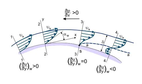
FIGURE 3.1: Development of the boundary-layer at an airfoil [17]
In an airfoil Outside the boundary layer, as can be seen from the figure, the
pressure p(x) increases with distance, since the pressure gradient ¶p
¶x in this direction
obeys Bernoulli’s equation:
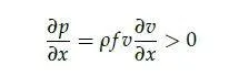
Since variations in pressure in the transverse direction are negligible, we find an
identical longitudinal pressure gradient within the boundary layer. Thus, in the
low-velocity regions near the wall, the dynamics of the fluid elements are affected
by two opposing effects; the positive pressure gradient ¶p
¶x slows down their motion
and also momentum transfer by viscous diffusion from higher velocity regions
accelerate them. If the velocity gradient ¶v
¶x is sufficiently large in magnitude
there will be a reverse flow near the wall. This phenomenon commonly is known
as boundary-layer separation.[18]
3.2 Governing Equation
By selecting a suitable turbulence model we can simulate Modified airfoil geometry
to generate data for aerodynamic forces. In the study of an airfoil, the
main objective is to get force coefficients. As the performance of an airfoil is mainly
a function of lift and drag coefficient. The objective of an airfoil design is to get
the maximum lift to drag ratio for its most efficient operation. The reason to find the
coefficient of lift and drag instead of its forces is to use this number to model all
the complex dependencies of any body shape.[19] As can be seen from the figure
below the point through which these aerodynamic forces act is known as the center
of pressure. The Center of pressure is the average location of the pressure in an
airfoil. The Center of pressure moves with the angle of attack.[20]
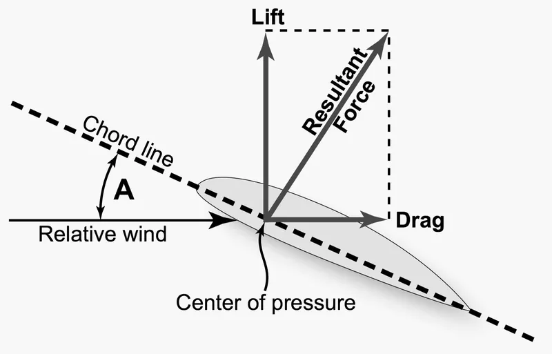
FIGURE 3.2: Aerodynamic forces in an airfoil [17]
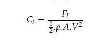
Coefficient of Lift (Cl) : (Cl) is a dimensionless coefficient that relates the lift
generated by a body to the density of the fluid (r) around the body, the velocity of a fluid
(V) and the wing area (A). Cl is a function of the angle of the body to the flow known
as the angle of attack, it is Reynolds number (Re) and its Mach number (M). The Coefficient
of lift refers to the dynamic lift characteristics of a two-dimensional foil
section, with the reference area replaced by the foil chord.[21]
The coefficient of lift (Cl) is defined as [22]
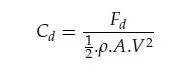
Coefficient of Drag (Cd): Drag force acts parallel to the airflow direction and
acts mainly due to the viscous friction force of the airfoil blade surface. To increase
the efficiency of any wind turbine to generate electricity we have to keep the lift
to drag ratio maximum. The coefficient of drag is a dimensionless quantity used to
quantify the resistance of a body in a fluid. The drag coefficient of any object consists
of mainly skin friction and form drag. The drag coefficient of a lifting airfoil or
hydrofoil also includes the effects of lift-induced drag.[23]
We can formulate the coefficient of drag as [21][22]
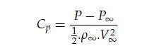
Coefficient of Pressure (Cp): Cp is the difference between local static pressure
and free-stream (at ¥) static pressure, nondimensionalized by the free-stream dynamic
pressure. At any point in the flow where the local coefficient of pressure
Cp can be formulated as [24]
3.3 Velocity Ratio in Rotating Cylinder
As stated earlier, the Lift and Drag coefficient varies with different speeds of rotation
of the cylinder. Hence, the velocity ratio (W) is the primary parameter control
to consider for the study.
The velocity ratio (W) is determined by non-dimensionalizing the cylinder peripheral
velocity by the free-stream velocity.
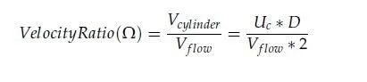
where,
Uc = Cylinder rotation in radians per second (rps),
Vf low = Velocity of fluid in meters per second (m/s),
D = Diameter of the cylinder in millimeter.
Increasing the velocity ratio creates a variation in the relative velocities around
the surface of the cylinder, giving rise to pressure asymmetries that are the chief
cause of the aerodynamic forces and moments acting on the cylinder.[25]
3.4 Conservation Laws of Fluid Dynamics
The conservation laws may be applied to a region of the flow called a control
volume. A control volume is a discrete volume in space through which fluid is
assumed to flow. The integral formulations of the conservation laws are used to
describe the change of mass, momentum, or energy within the control volume.
Conservation of Mass (The continuity equation): To understand how aerodynamic
forces arise, the basic principle of conservation of mass must be considered. Conservation
of mass states that mass can neither be created nor destroyed. This
principle can be easily described using the model of an ideal fluid, one that is
inviscid, or has zero viscosity, and is incompressible. “The continuity equation
is a statement of the conservation of mass in a system. The continuity equation
states that the fluid “mass flow rate” the amount of fluid per unit time must be
the same at any cross-section of the pipe or else there is an accumulation of mass
“mass creation” and the steady flow assumption is violated.”[5]

Conservation of Momentum (Navier-Stokes equation): Newton’s second law of
motion applied to a control volume is a statement that any change in momentum
of the fluid within that control volume will be due to the net flow of momentum
into the volume and the action of external forces acting on the fluid within the
volume.
The Navier-Stokes equations are the fundamental partial differentials equations
that describe the flow of incompressible fluids. As we have stated earlier
currently the majority of the model which analyze more and more complex fluid flow
the pattern is based on the incompressible Reynolds-Averaged Navier-Stokes equations
(RANSE) which is derived from newton’s second law of conservation of
momentum as stated below:

3.5 Turbulence Model
The method used to predict the turbulent flow behavior is Reynolds averaging of
Navier-Stokes equation which introduces a new variable called Reynolds stress
tensor. Reynolds stresses must be modeled to close the system of governing equations.
These additional stresses are modeled using eddy viscosity or turbulent
viscosity (m).
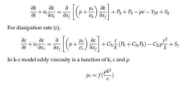
3.5.1 k-epsilon model
k-# turbulence model is widely used in practical industrial applications. k-# turbulence
the model uses two extra transport equations to represent turbulent flow,
namely turbulent kinetic energy (k) which represents energy in the turbulence
and energy dissipation rate (epsilon) which represents the scale of the turbulence. This
model is used mainly in planar shear flow and recirculating flow but performs
poorly in large adverse pressure gradient, curved boundary layers, and rotating
flow. Transport equations for the standard k-epsilon model are:
For turbulent kinetic energy (k),
3.5.2 kw-SST model
The K-omega model also uses two equations to represent the turbulence, but instead
of e, it calculates a specific turbulence dissipation rate, which can be considered
the ratio of e to k. [26]
kw-shear stress transport (SST) model is a combination of standard k-epsilon
model and k-omega model. The model depicts the behavior of flow near-wall boundary
using the Wilcox kw model and for flow away from the wall using the standard
k-# model, using blending function. The blending function is designed to be one
in the near-wall region, which activates the standard kw model and zeroes away
from the wall, which activates the standard k-# model. This model is suitable for
adverse pressure gradient and flow separation. This model depends on the wall
the distance which makes it less suitable for free shear flows. Transport equations
for turbulent kinetic energy (k) are the same as the k-epsilon model and for specific
dissipation rate (w),
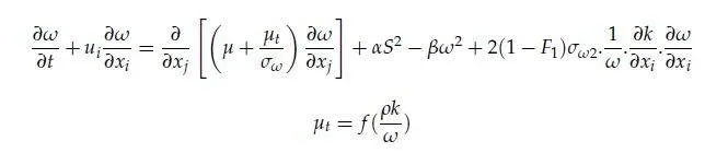
In the kw-SST model, eddy viscosity is a function of k, w, and rho.
3.6 Techniques for Modeling Flows in Moving Zones
The task of thesis work is to model a flow around a modified airfoil that has
a cylinder attached to it. The cylinder is placed at the leading and trailing edge of
an airfoil. There are different approach to solve a problem involves moving parts.
In this thesis two of these approach has been used to model flow in moving zones.
3.6.1 Rotating Wall Method
In rotating wall method can be specified in a flow with a stationary reference
frame. In ANSYS Fluent this option is enabled by selecting a moving wall under
the boundary condition. The types of motion need to be given as per the task
such as rotational or translation motion. Then after the Axis of rotation of a body
needs to be given. The rotating wall approach considers the mesh around the
rotating body as frozen and no-slip condition enables flow to model in the reason
around the rotating part of a geometry.
This approach considers two regions with one as a rotating framework and
another as a stationary framework. The solutions from both regions are matched
at the interface between the rotating and stationary regions via velocity transformation
from one frame to the other. This velocity-matching step involves the
implicit assumption of a steady flow condition at the interface.[27]
The rotating wall approach is suitable for steady-state problems. This technique
saves time of simulation and hence cost-effective to use. This method uses relative
motion to the adjacent cell zone as the wall is rotating hence its motion effect
transfers to the nearby mesh.
3.6.2 Sliding Mesh Approach
"In the Sliding-Mesh approach, full transient simulations are carried out using
two grid zones. One of the grid zones is attached to the rotating region while
the other grid zone is attached to the stationary region. This approach involves
mesh motion, hence it is imperative that the interface between the zones be two
overlapping faces, one of which is attached to the rotating region while the other
is attached to the stationary region. The interaction between the two regions is
modeled by interpolating the information across these faces."[27]
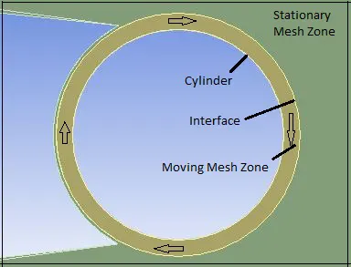
FIGURE 3.3: Sliding Mesh Approach
As can be seen from the figure above sliding mesh involving two mesh zone
close to each other. In a sliding mesh approach, the simulation is transient as
it involves mesh motion. The computational time is very high and hence this
method is very costly. This approach is suitable for the model where rotating and
steady parts are close to each other in a geometry. The sliding mesh technique
gives better accuracy compares to other approaches while simulating a model
involving rotating parts.
3.7 Joukowsky Airfoil
The Russian scientist Nikolai Egorovich Joukowsky studied the function
J(z) = z + (1/z)
He showed that the image of a circle passing through and containing the point
is mapped onto a curve shaped like the cross-section of an airplane wing. This
curve is known as the Joukowski airfoil.[28]
Variation in the thickness of the profile can be achieved by a small displacement
of the center of the transformed circle in the direction of the abscissa; camber
in the airfoil is obtained by a small displacement of the center in the direction of
the ordinate.[29]
The solution of the flow around a circular cylinder with circulation in a cross
flow can be used to predict the flow around thin airfoils. We can transform the
local geometry of the cylinder into an ellipse, an airfoil, or a flat plate without
influencing the geometry in the far-field. This procedure is known as conformal
mapping. [30] The figure below shows the transformation of a circle into an airfoil
by using the Joukowsky function.
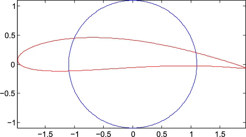
FIGURE 3.4: Mapping of a circle to an airfoil [30]
This thesis work uses a 15% thick symmetric Joukowsky airfoil as a base airfoil.
Many experiments are performed over a modified Joukowsky airfoil to study the
Magnus effect. The simple design and profile of a Joukowsky family of an airfoil
help in its better modification which eventually provides bases for the study of
the Magnus effect. 15% thickness is suitable to fits in the cylinder which has a
sufficiently large diameter which helps in a better fluid flow over the entire surface
of an airfoil. The profile of an airfoil can be seen below.
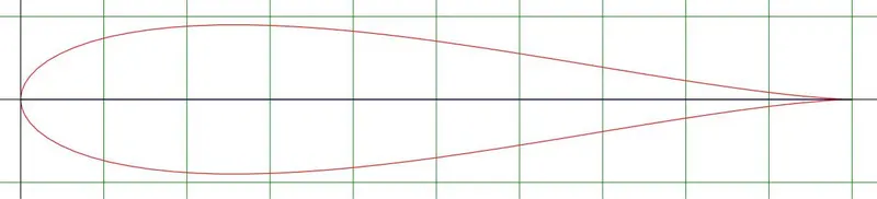
FIGURE 3.5: Joukowsky 15% thickness airfoil
Chapter 4 Implication of Magnus effect on Wind Turbine Aerodynamics
As stated in earlier sections about the potential of the Magnus effect to generate
significant lift and also about the previous work done on its practical implication
to the modern wind turbine.
This chapter deals with the actual design of a model by modification of a
Joukowsky airfoil with the different sets of a cylinder, it also includes ANSYS
fluent setup and initial and boundary parameter input section.
4.1 Modified Airfoil Geometry
From the literature review and studies from the former research papers, it is evident
that out of the numbers of possibilities for the placement of cylinder on the
edge of an airfoil, most efficient and significant results are obtained by placing
the cylinders at the extreme edge on either side of an airfoil. As can be seen from the
figure below from the previous works the geometry can be modified as per these
dimensions to have better results for comparison. This thesis work uses those
two different sets of geometry namely leading edge and trailing edge cylinder.
As the study requires basic 2D sketching, ANSYS “design modular” is a more
feasible option to use for making geometry.
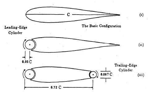
FIGURE 4.1: Various Rotating Cylinder Configurations [1]
4.1.1 Leading-Edge Cylinder
The Leading-edge cylinder as shown in the figure keeps the overall configuration of
geometry quite similar to the normal airfoil. To make geometry in ANSYS design
modular, first, there needs to change the .txt file of an airfoil. The point of an
airfoil which makes for the leading edge needs to be removed. For this thesis
work, chord length is shortened by around 10% to fit the cylinder. The chord length of
the original airfoil is 370mm and the diameter of a cylinder is 13 mm. To replicate
the real-life effect, there is a gap of around 1.2 mm between cylinder and airfoil.
The diameter of the cylinder is select in such a way that (choose such that) overall
geometry replicate an airfoil-like shape. This will ensure the smooth flow of a fluid over
the surface of the cylinder and airfoil.
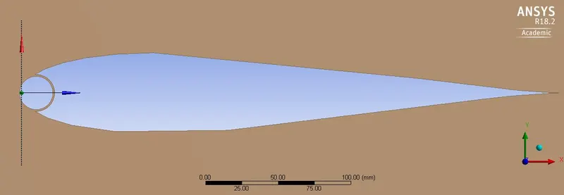
FIGURE 4.2: Leading-edge rotating cylinder geometry
From the above geometry, it can be seen that all the domains of fluid act as
stationary domains and as a single zone. This geometry is for the rotating wall
method as it does not require splitting the rotating zone and stationary zone.
Geometry for Sliding Mesh Approach: For the sliding mesh approach the
remaining procedure to make a model is the same as above. The only difference is to
make another circular domain around the cylinder to make it a rotating zone.
This procedure splits the whole fluid into two parts but acts as a single unit during
the simulation. The connection between the two domains is known as the interface.
The geometry for the Leading edge cylinder with sliding mesh approach
can be seen from the figure below.
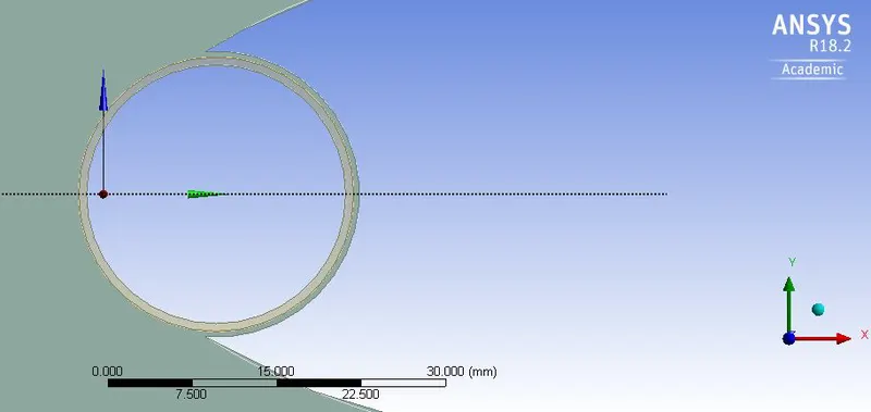
FIGURE 4.3: Leading-edge cylinder geometry for sliding mesh approach
4.1.2 Trailing-Edge Cylinder
Unlike the previous configuration, the trailing edge cylinder shortens the overall length
of an airfoil. To generate this model the .txt file of an airfoil plotter is edited
to remove points of a trailing edge. After cutting out trailing edge points, the
edge needs to be connected by an arc or a curve shape line in the design modular.
For better configuration of geometry, this arc should have the same geometrical
center as the cylinder. These will make a good model with a constant gap
between the airfoil and the cylinder. The diameter of a cylinder here is 26 mm.
The geometry with a trailing edge cylinder for rotating wall approach is as shown
in the figure below.
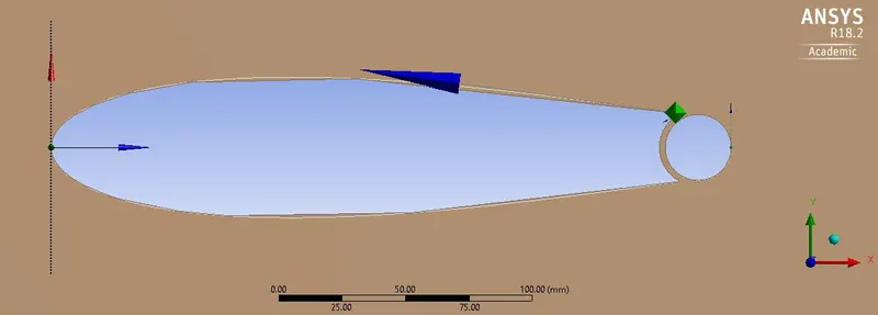
FIGURE 4.4: Trailing edge rotating cylinder geometry
In trailing edge configuration the overall length of an airfoil is reduced to
270mm from 370mm chord of a base airfoil. This reduction in length is necessary
to provide a cylinder with a large enough diameter which makes for a significant
effect on the overall result.
Geometry for Sliding Mesh Approach: Similar to the previous method, to
make geometry for a sliding mesh approach the zone around a cylinder needs to
be separated from the stationary zone. These separate zones then help in providing
rotation to the cylinder zone fluid to better capture the effect of force generation
due to rotation. The geometry for this approach as shown below is similar to
that of the rotating wall approach with two separate zones, unlike in the former
case.
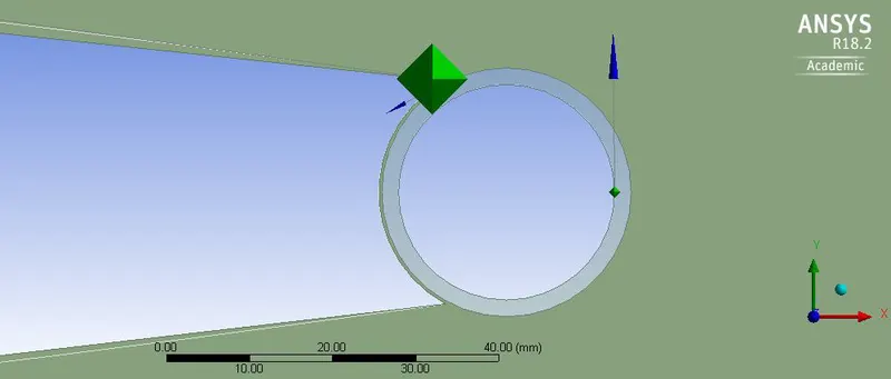
FIGURE 4.5: Trailing edge cylinder geometry for sliding mesh approach
4.1.3 Geometry of a Fluid Domain
After creating an airfoil profile it is necessary to generate a fluid domain around
it for capturing all the turbulent effects around the airfoil. This control volume
should have enough size so that it can give accurate simulated results. This
computational domain is necessary for every fluid simulation in fluent to capture
the far-field effect.
Steps to create c-mesh domain around the Modified airfoil geometry :
• Create a circular arc with radius 10 times the chord length (i.e. 3700mm) for
the inlet section.
• Outlet section is far away at the distance of 12 times the chord length
(i.e. 4440mm).
• The rectangular outlet section is created as shown in the figure below.
• These domain sketch is then converted to lines to further specify it as
physical boundaries.
• Geometry of a cylinder and airfoil is then frozen using the tool to make it as
separate entities.
• Lines of a domain is then converted to surface which will act as a fluid
during simulation.
• Then after the surface of an airfoil geometry needs to be subtracted from the
fluid surface by using the Boolean tool in the design modular.
The C-mesh domain with all the dimensions is as shown in the figure below.
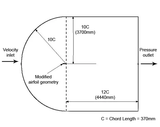
FIGURE 4.6: C-Mesh Domain
In the case of sliding mesh approach model geometry, all of the procedures
are as stated above except in this case the whole fluid domain is converted into
two parts. The stationary part is defined as the outer fluid and the rotating fluid zone
around the cylinder is defined as the inner fluid. This approach is the same both in
the case of a leading-edge as well as a trailing edge cylinder.
4.2 Meshing of an Airfoil Geometry
After creating model geometry and fluid domain around its next step is to discretize
the domain for simulation. The meshing of geometry can be done using
a number of available tools in Ansys. This thesis study deals with the ANSYS
Meshing for meshing of a geometry. As in this thesis, geometry is 2-D, it is feasible
to use ANSYS Meshing. This tool is easy to use for simple geometry as well
as have good tools and options for both structured and unstructured meshing.
Reason for the Unstructured Meshing: The model used in this thesis is as
shown in former sections has very sharp edges around the corner of and cutout
airfoil section. Also, the gap between the cylinder and the airfoil surface is quite
narrow. This kind of geometry requires a very careful meshing procedure. Structured
meshing in such a model is very difficult to achieve and also very time-consuming.
Hence, this kind of geometry is discretized using unstructured
meshing. After reading through numbers of research work related to the same
task performed here, it is evident that unstructured meshing gives good results
and it is easy to generate compared to other meshing tools and procedures. Below
stated are the procedure done on ANSYS meshing to generate grids in the
geometry.
Steps to create unstructured meshing around the geometry :
• Before generating the mesh, few default details need to change under meshing
section such as sizing and physical preferences.
• Physics preference needs to be selected as CFD.
• Select Fluent under the solver preference.
• After that, it is necessary to give details regarding the sizing of a grid and
other properties such as inflation layer setting and defeature sizing under
the "Sizing" section.
• After initial settings, the next step is to give edge sizing to the different edges
in the geometry.
• In case of the sliding mesh approach, it is also required to give face sizing to
the rotating part, which generates fine meshing around the cylinder which
is an important part of the model.
• After providing all the sizing, the next step is to provide a triangular method
to the whole body. This will generate unstructured triangular elements in
whole geometry.
Mesh Independency: Mesh independency states that after a certain number
of elements the output of a results does not affect greatly hence it is not necessary
to create a grid more than that point, which saves computational time as well
as cost and provides the best result by consuming fewer resources. The figure below plots
the results of a simulation for a 6-degree angle of attack and a velocity ratio
of 2, for different numbers of elements with trailing edge cylinder geometry. As
can be seen that the coefficient of lift does not get the effect after around 100k grid
points. hence, to get a good result it is not necessary to generate a mesh with
approximately 100k grid elements.
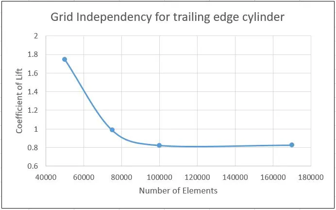
FIGURE 4.7: Mesh independency test for trailing edge cylinder geometry
Similarly for the leading edge cylinder geometry also above procedure is followed
to check optimum grid element numbers. In this case numbers of tests are
performed for an 8-degree angle of attack and velocity ratio of 1. From the figure,
it can be concluded that the minimum numbers of elements require for good
results in this geometry is around 200k.
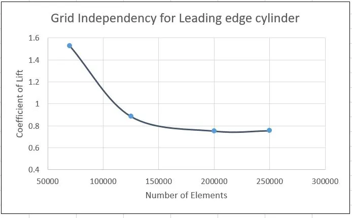
FIGURE 4.8: Mesh independency test for leading-edge cylinder geometry
After following all the steps as stated ahead, meshing is generated in the model.
To have good results of a simulation, meshing in a critical area such as airfoil
and cylinder wall as well as edges gap between the airfoil and cylinder needs
to carefully handle. The figure below shows the meshing in leading-edge cylinder
geometry.
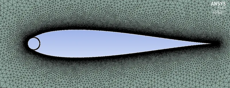
FIGURE 4.9: Meshing of leading-edge cylinder geometry
As can visualize there is very dense meshing nearby the surface of a cylinder
and airfoil. For better capturing the effect of flow over the surface of the airfoil, it is
necessary to keep meshing very fine in that region of interest.
The meshing for the sliding mesh approach is also similar to that of normal
geometry with the only difference being, there is additional face meshing around the
cylinder. This part needs to carefully mesh as it has an interface with the stationary part
of a fluid domain, hence these transition needs to be smooth for the good quality
result. An enlarged section of an interface between rotating and stationary parts is
shown in the figure below.
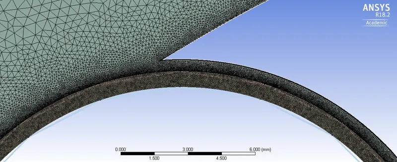
FIGURE 4.10: Meshing of leading-edge cylinder geometry for sliding mesh approach
The edge of an airfoil part is split into half horizontally by using "split-edge"
tool. This step needs to be done before applying edge sizing, this splitting of
an edge will ensure smooth and attached meshing around the curve of an airfoil
section.
By following a similar process as done earlier for the leading edge cylinder
geometry, meshing for the trailing edge cylinder geometry is achieved. This in fact
has less complication compared to the former case as trailing edge cylinder
geometry does not have a sharp trail edge which makes the meshing process
easier. below is the figure for the mesh of trailing edge cylinder geometry.
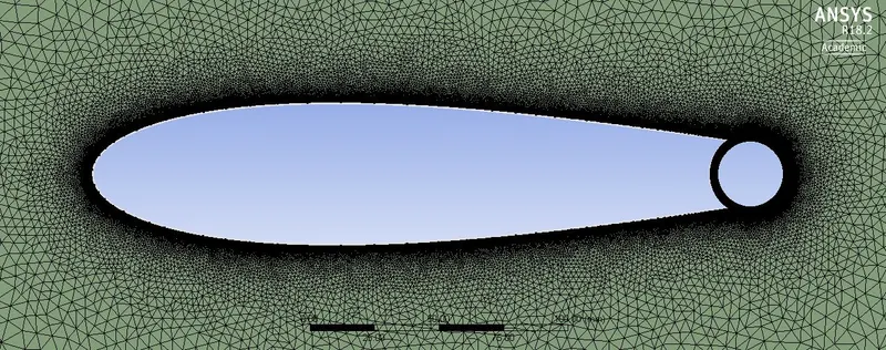
FIGURE 4.11: Meshing of trailing edge cylinder geometry
The figure below shows the meshing section around the rotating part of a trailing
edge cylinder and the stationary part. As can be seen from the figure below
the transition between rotating and stationary parts is smooth, which will ensure
the better transfer of physical quantity during the process of simulation.
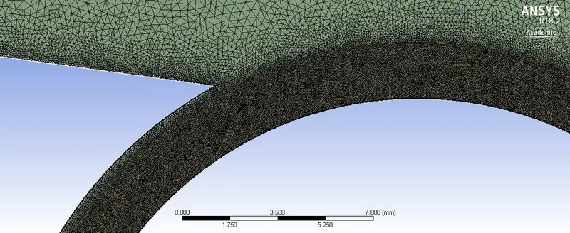
FIGURE 4.12: Meshing of trailing edge cylinder geometry for sliding mesh approach
4.2.1 Name selection in geometry
After generating meshing throughout the model, the next step towards simulation
is the name selection. This step needs to be carefully handled as ANSYS
The fluent tool is very name sensitive.
For rotating wall geometry: In the rotating wall approach naming is relatively
easier for the model compared to the sliding mesh approach. For both the leading
edge cylinder and trailing edge cylinder name selection is similar.
• Inlet: Inlet boundary is given by selecting the edge selection tool and picking
up 3 edges as shown in the figure below.
• Outlet: Outlet boundary is the far left boundary as shown in the figure.
• Airfoil: Airfoil wall is consist of modified cutout airfoil as well as arc joining
the two end of the modified airfoil.
• Cylinder: The Cylinder wall is given by picking up a cylinder surface from
edge tool.
• Fluid: Fluid is naming to the whole surface of the domain by using the face
selection tool as shown below.
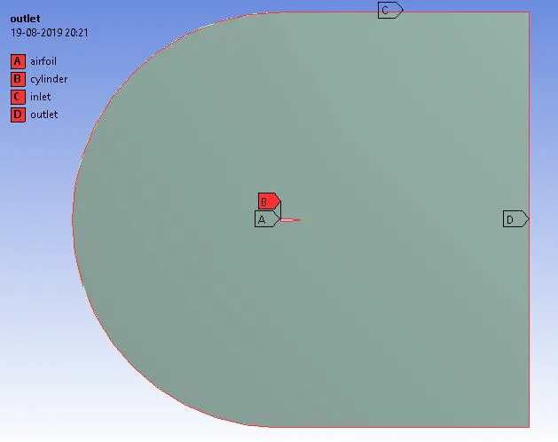
FIGURE 4.13: Name selection in model
In the above figure, all the area within the domain seen as grey is the fluid domain.
ANSYS fluent automatically consider all the domains without any name as the fluid
domain. Hence, sometimes it is not necessary to specify the fluid domain separately
in name selection.
As can be seen from the above figure it is not visible the boundary of the cylinder
and airfoil, hence it is magnified in the figure below to show the exact surface of
those components. The figure below is an enlarged section showing the actual
geometry of a cylinder and an airfoil with named selection.
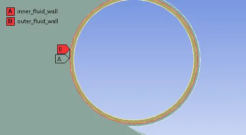
FIGURE 4.14: Enlarged section with Name selection
For the sliding mesh approach: In the sliding mesh approach the only difference
from the above process is regarding the fluid domain. In this case, two different fluid
domain is created. One is rotating and the other is stationary.
• Inner_fluid: Inner fluid name is given to fluid surrounding the rotating
cylinder by picking the face selection tool.
• Outer_fluid: Outer fluid is stationary fluid in the whole other remaining domain.
• Inner_fluid_wall: By suppressing the outer fluid domain and picking up the
edge tool, the outer wall of the rotating domain is named as the inner_fluid_wall.
• Outer_fluid_wall: Similarly by suppressing the inner fluid domain and picking
up the inner edge of a stationary domain, it is named as the outer_fluid_wall.
FIGURE 4.15: Name selection for sliding mesh approach
4.3 Statistics and properties of a mesh
After creating a mesh in geometry it is necessary to check all the statistics and
properties of the mesh before running simulation. Good quality of the mesh is
important for good simulation and appropriate output results. There are several
parameters to check the quality of the unstructured mesh, this thesis work has only
considered parameters with prime importance namely orthogonal quality, aspect
ratio, and skewness.
4.3.1 Leading-edge cylinder geometry
Leading-edge cylinder geometry has the following stats after completing the meshing
process.
• Number of elements: 475400 elements
• Number of nodes: 253250 nodes
The below figure shows the histogram plot of an orthogonal quality matrix of a
mesh for a leading-edge cylinder geometry.
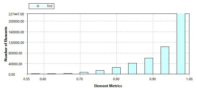
FIGURE 4.16: Orthogonal quality matrix of leading-edge cylinder geometry
Properties of the orthogonal quality matrix :
• Minimum value: 0.55488
• Maximum value: 1.0
• Average value: 0.92888
For the worst cell, orthogonal quality is close to 0 and for the excellent cell, it is
close to 1. In an orthogonal quality matrix, the permissible limit for excellent
quality is within the range of 0.95-1. From the above graph and statistics, it is
evident that mesh has a good orthogonal quality value as an average value of 0.92888
lies in a very good quality region.
The curve below shows the aspect ratio matrix for the mesh of a leading-edge
cylinder geometry.
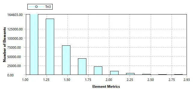
FIGURE 4.17: Aspect ratio matrix of leading-edge cylinder geometry
Properties of aspect ratio matrix :
• Minimum value: 1.0001
• Maximum value: 2.9297
• Average value: 1.3385
From the above curve and stats, it can be seen that the aspect ratio of a mesh is
also very good and acceptable for further simulation.
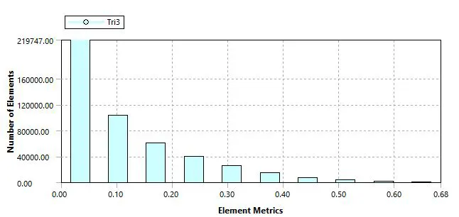
FIGURE 4.18: Skewness matrix of leading-edge cylinder geometry
The curve shown ahead is a curve for a skewness matrix of a mesh for the leading edge
cylinder geometry.
Properties of skewness matrix :
• Minimum value : 2.8769e-08
• Maximum value: 0.68362
• Average value: 0.11565
For good skewness of a mesh, the value needs to be within an excellent permissible
range of 0 to 0.25. Hence, from the above curve and statistics, it can be seen that
mesh has very good skewness.
From all the above stats and properties it can be concluded that the leading
edge cylinder has a good quality of meshing and can further proceed for the
simulation process.
4.3.2 Trailing-edge cylinder geometry
Trailing-edge cylinder geometry has the following stats after completing the meshing
process.
• Number of elements: 356738 elements
• Number of nodes: 188771 nodes
Similar to the case of a leading-edge cylinder, for this geometry also there is quality
checking for parameters such as orthogonal quality, aspect ratio, and skewness.
The below figure shows the histogram plot of an orthogonal quality matrix of a
mesh for a trailing edge cylinder geometry.
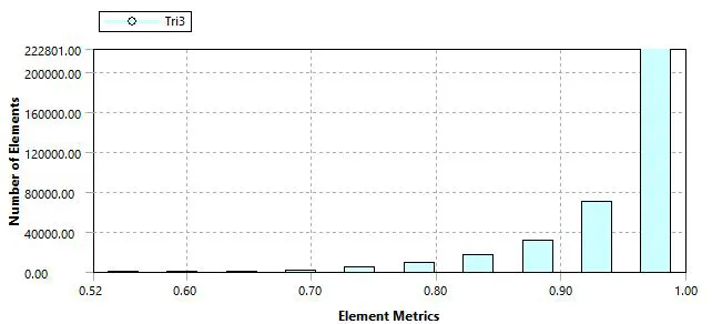
FIGURE 4.19: Orthogonal quality matrix of trailing-edge cylinder geometry
Properties of the orthogonal quality matrix :
• Minimum value: 0.52464
• Maximum value: 1.0
• Average value: 0.94787
As stated earlier, in the orthogonal quality matrix, the permissible limit for the
excellent quality is within the range of 0.95-1. From the above graph and statistics,
it is evident that mesh has a good orthogonal quality value as the average value
0.94787 lies in a very good quality region.
Aspect ratio is defined as the ratio of asides of an element of a mesh cell.
For good quality of the mesh, it is necessary to have a value of aspect ratio close to
1. As high aspect ratio means either to long mesh cell or a very small aspect ratio
means the volume of a cell is almost zero which is not physically permissible
for simulation. The curve below shows the aspect ratio matrix for the mesh of a
trailing edge cylinder geometry.
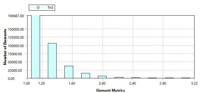
FIGURE 4.20: Aspect ratio matrix of trailing edge cylinder geometry
Properties of aspect ratio matrix :
• Minimum value: 1.0001
• Maximum value: 3.2154
• Average value: 1.2669
From the above curve and stats, it can be seen that the value of aspect ratio is
very good for all the cells in the meshing geometry. Hence, aspect ratio wise also
trailing edge cylinder geometry meshing is also excellent for further simulation
procedures.
After checking for the orthogonal quality and aspect ratio, the final check is
for the skewness in the cell for the trailing. The next curve shows the skewness
matrix of a meshing.
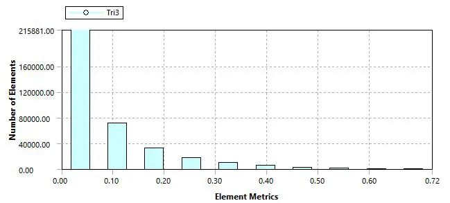
FIGURE 4.21: Skewness matrix of trailing edge cylinder geometry
Properties of skewness matrix :
• Minimum value : 2.9513e-08
• Maximum value : 0.72302
• Average value : 8.4778e-02
As stated earlier, for good skewness of a mesh the value needs to be within an excellent
permissible range of 0 to 0.25. Hence, from the above curve and statistics, it
can be seen that mesh has very good skewness.
From all the above stats and properties it can be concluded that the trailing
edge cylinder also has a good quality of meshing and can further proceed for the
simulation process.
4.4 Solution methods and Numerical Scheme Setup
Once a good quality mesh has been generated throughout the model and name
the selection has been done, the next step is to input these mesh file into ANSYS
Fluent solver.
To compare the solution with experimental results it is necessary to provide
physical condition the same as that of the experimental case. Before starting simulation
it is necessary to provide all the initial setup in the solver. This section
shows all the initial conditions and numerical scheme setup steps for various
case studies of this thesis work.
The initial setup for both the leading-edge cylinder and trailing edge cylinder is
quite similar. However, it is somewhat different for the rotating wall approach
and moving mesh approach. In this section below there is an overview regarding
all the initial setup before stating the simulation for both the approach separately.
To get speed up in the simulation process select double precision and if possible,
use a parallel computing option before initializing fluent solver.
Numerical scheme setup for rotating wall method :
Before running the simulation, the general initial setup needs to be done in the
fluent solver. For the rotating wall method, simulation is the Steady-state and the
solver used is Pressure-Based.
Turbulent Model: The Turbulent model for this case is mainly K-# and Kw-SST
chosen from Models option and then Viscous models.
Materials: The fluid used in this setup is Air which has the following properties.
• Density : 1.225 kg/m3
• Viscosity : 1.7894e-05 kg/ms
Cell Zone Conditions: For the rotating wall approach cell zone has a whole
domain as fluid and it is kept stationary with air is chosen as material.
Boundary Conditions: Boundary condition has various sections of a geometry
namely airfoil, cylinder, inlet, outlet, and fluid.
In the airfoil section, specify it as a Wall and choose Wall motion as stationary.
Choose No-slip condition under Shear condition options. Keep Roughness Models
as a Standard under the Wall roughness section and provide Roughness constant
value 0.5.
In-cylinder section, specify Wall motion as moving wall. After that in the Motion
part select Motion "Relative to Adjacent Cell Zone" and types of motion as "Rotational".
Provide speed of a cylinder in Radians per second. For clockwise rotation
as in this case, it is necessary to give negative signs before rotation speed. Give
Rotation-Axis origin value under that section as per the geometry of a model.
In our model Axis of Rotation for the Leading-edge cylinder is (0.01m, 0m) and for
the trailing edge cylinder, it is (0.255 m, 0m). Similar to the airfoil, choose No-slip
the condition under Shear condition options. Keep Roughness Models as a Standard
under the Wall roughness section and provide Roughness constant value 0.5.
The table below shows the value of the rotational speed of cylinder (In Radians
per Second) for different velocity ratios both the geometry.

In the inlet section which is Velocity Inlet, choose Velocity Specification Method
as "Magnitude and Direction". Specify velocity as calculated from Reynolds's number.
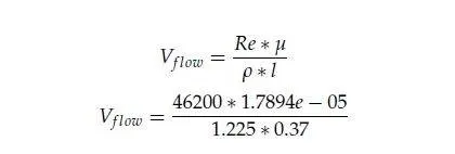
Hence, the velocity of flow is 1.823944 m/s.
The angle of attack can be specified under the X and Y component of a flow direction
by calculating the sine and cosine value of an angle.
In the outlet section which is Pressure outlet, choose Gauge pressure as 0 pascals.
Solution Methods: In the solution method section under pressure velocity coupling
choose scheme as Coupled. Specify all spatial discretization as Secondorder
upwind for the fast convergence of a solution.
Solution Controls: Under the solution control section specify Flow Courant Number
as per the setup and method. Specify Explicit and Under-Relaxation factors
for the controlling speed and accuracy of the solution.
Report Definitions: In the report definitions section create two force report files
for the Lift and Drag coefficient. This file will provide output data of force after
completion of a simulation.
Residual Monitors: Residual is an important parameter to be specified before
the final run of a simulation. Smaller residuals value will give better and accurate
results but it will take high computing time. Hence, it is necessary to choose
residuals as optimum to give better results within the scope of a time. This thesis
work uses a 10e-05 order of residuals for the simulation.
After specifying all the above initial parameters and values for the setup, the case
is ready to run for simulation after Solution initialization. There are two methods
for solution initialization namely Hybrid and standard. As per the case requirements
method is chosen and the case is stared for simulation. The number of
Iteration needs to be provided in the calculation section before running the simulation.
Numerical scheme setup for sliding mesh approach :
The numerical scheme set up for the sliding mesh approach is slightly different
compared to a moving wall approach. Although numbers of initial setup is similar
to that approach. In this part, only parameters that differ from the above
approach are discussed in length. Unlike the previous case, this approach runs
on the Transient simulation method as it involves rotation of mesh.
Cell Zone Condition: In this approach cell zone is consists of two parts, inner
fluid, and outer fluid. The outer fluid is kept stationary as in the previous case while
the inner fluid is given as mesh motion. The rotation parameter of this zone depends
on the velocity ratio and cylinder speed. Also, the axis of rotation is the same as
that of the axis of rotation for the cylinder.
Mesh Interface: As there is two domain within the continuous fluid zone it is
necessary to create an interface between the two domain. From the boundary condition
section select Inner_fluid_wall and Outer_fluid_wall. Specify these two as
an "Interface" instead of "Wall". This will create a new section of Mesh Interface.
Then under the mesh interface section create a new interface by selecting these
two boundaries.
The remaining procedure for the setup is the same as the previous case until
the running of an actual simulation. As this case runs on a transient time step
approach it is necessary to provide an appropriate time step size before running
the case.
Time step size selection :
For transient flow simulation, the time step size is one of the important parameters.
Choosing the correct time step size is very important, as too small a time step
leads to more time-consuming simulation which increases computational costs.
A very small step affects the accuracy of the solution. Hence, it is necessary to
choose optimum time step size and number of iterations per time step size to
have accurate as well as resource-saving simulation results.
In this thesis work time, the step size is selected after studying the effect of various
time steps. As the scheme used is the current task is fully implicit, the Courant
number can be allowable up to 10, 20, or even up to 100. CFL (Courant-Friedrichs-
Lewy) condition is one of the important parameters to be considered for the accuracy
and stability of transient simulation.
CFL criteria can be defined as :

Where,
C = Courant number,
U = Effective velocity of flow,
D t = Time step size,
D x = smallest grid size.
In this task time, the step size is selected such that the cylinder rotates about 1o for a
one-time step size. Although this selection leads to a time-consuming simulating
process it was necessary for comparison study and also better to implement
as the numbers of simulations performed with this process were limited.
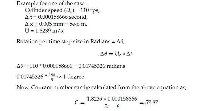
As this time step size is smallest in this task study and Courant number is within
the permissible limit for this case, it is evident that for all other cases CFL number is
within acceptable limits for accurate results.
Chapter 5 Results and Discussion
After completing all the setup and simulation in a fluent solver, there are aerodynamic
force data collected which determine the effect of modification of airfoil
geometry. These data will also help in comparing the base airfoil to the modified airfoil.
This comparison will prove how the Magnus effect is affecting the base airfoil
and how different cylinder speeds and cylinder arrangements affect the aerodynamic
properties of an airfoil.
This section is comprised of all the results from the base Joukowsky airfoil as well
as different arrangements of geometry after modification. This chapter also consists
of a comparison of various geometry and methods as well as a comparison
of different operating conditions on the output of an airfoil.
5.1 Aerodynamic properties of Base Joukowsky Airfoil
Before comparing results of various modified geometry it is necessary to see how
base Joukowsky airfoil with 15% thickness behaves in similar operating conditions.
The coordinate data file of a Joukowsky airfoil model is generated in ANSYS
design modular as shown in the figure below. Similar to the modified geometry
concept after sketching airfoil, it is necessary to create a fluid domain as discussed
in the previous chapter for further simulation process.
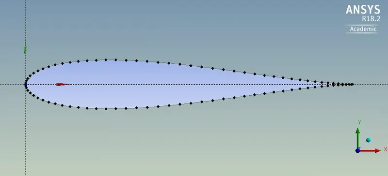
FIGURE 5.1: Sketch of base Joukowsky airfoil in Design modular
After creating model geometry the next step is to generate meshing in an airfoil.
As this model is simple it is appropriate to create structured meshing using the ICEM
tool. Figures below show the meshing of the full fluid domain as well as an enlarged
portion showing structured mesh around the wall of an airfoil.
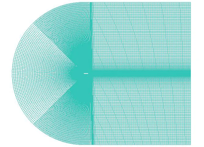
FIGURE 5.2: Meshing of base Joukowsky airfoil in ICEM tool
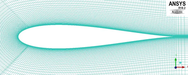
FIGURE 5.3: Enlarged portion of meshing around the airfoil
After the discretization of a domain, the model is imported to a Fluent solver
for simulation. To have a better comparison with experimental results it is necessary
to have some physical condition setup before running simulation. In the
experimental results of our concern, the Reynolds number is kept around 46200 [1].
As calculated in the previous chapter to achieve this value of Reynolds number,
the velocity of flow is 1.82395 m/s. The viscous model used for the simulation is k-#
the turbulent model gives accurate results for the near-wall effect compared to another viscous model.
For comparison of the result generated from the simulation, there are X-foil
results as well as results from the experimental data of a research paper [1]. The
below figure shows the comparison of simulated results of this study with X-foil
results collected at 50000 Reynolds number and experimental results.
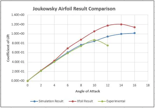
FIGURE 5.4: Comparison of lift data for base Joukowsky airfoil
From the graph above it can be seen that simulated results from the fluent are
very closely matched with experimental results. The deviation from the experimental
results at a higher angle of attack can be justified by the fact that experimental
results are generated from the setup of a wind tunnel, which is near impossible
to replicate in a simulated environment and other physical factors which
affects in experimental setup are not present in case of simulation.
5.2 Analysis of Airfoil with Leading Edge Rotating Cylinder
After validating the simulated result of a base airfoil, the next step is to see the effect
of the leading-edge rotating cylinder on the aerodynamic properties of a model.
In this study as discussed in a previous chapter different rotation ratio of a cylinder
is used to study the effect of speed of a cylinder.
Effect of Gap Between Cylinder and Airfoil: One important parameter to
be considered before finalizing the model is the gap between cylinder and airfoil.
The gap between the rotating cylinder and airfoil is of prime importance as this
can adversely affect the physics of a simulating model. Hence, it is necessary to
choose the optimum gap between the two entities. Numbers of research paper
and studies regarding moving surface boundary-layer control on airfoil surface
by rotating cylinder suggest that this gap should be around 1 to 2 mm for airfoil
length of around 300 mm and cylinder diameter around 25 to 30 mm [1] [2].
Considering the above-discussed aspect from various literature, this study
commences with different geometry of leading-edge rotating cylinder with varying
gap sizes between the cylinder and airfoil edges. After creating a model and generating
a mesh for 3 different geometries with a gap size of around 1.2mm, 1.5mm and
3mm; these models are run through a simulation for velocity ratio 4 and varying
angle of attack. The choice of this velocity ratio is totally random just to see the clear
difference between various models.
The figure below shows the curve of the lift coefficient against the angle of attack at
the spin ratio of 4 for different models.
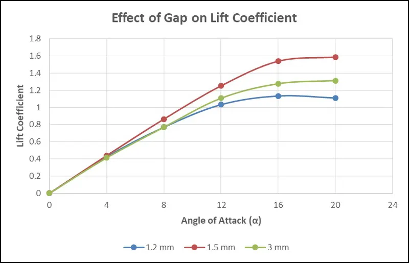
FIGURE 5.5: Effect of different gap size on Cl for leading-edge cylinder
The figure below shows the curve of the drag coefficient against the angle of
attack at the spin ratio of 4 for different models.
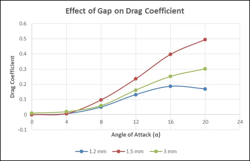
FIGURE 5.6: Effect of different gap size on Cd for leading-edge cylinder
From the graphs of lift and drag coefficient of various models, it can be clearly
visualized that too small or too large a gap has an adverse effect on aerodynamic
forces. From the graph, it can be seen that the model with a 1.5mm gap shows excellent
lift generation compared to other models with a gap of 1.2 mm and 3 mm. Although
the drag coefficient is small for a 1.2 mm gap compared to other cases but as
values of drag are on the smaller side this difference has little or no effect on overall
lift to drag ratio.
For model with a 1.2mm gap, this drops in force value especially at a higher angle
the attack is due to the small gap size which does not allow flow to smoothly transfer
from cylinder surface to airfoil surface.
For a model with a gap of 3 mm, a large gap in the model acts as a step from cylinder
to the airfoil for the incoming flow, which results in a large separation bubble
causing a decrease in lift coefficient as well as the effectiveness of a leading-edge
rotating cylinder. [1]
Hence, it can be concluded from the above study that a 1.5 mm gap is optimum
for leading-edge cylinder geometry in this study. All the simulations hereafter in
this paper performed over this model.
Aerodynamic properties of leading-edge cylinder geometry: The figure below
is plotted for lift coefficient against the angle of attack for the different spin ratio of
a cylinder. As leading cylinder geometry has a similar shape and physic with a normal
airfoil profile it behaves similarly to the base airfoil for small angle of attack
and even for small spin ratio. As can be seen from the curve spin ratio of 1 gives
very similar results to that of a base airfoil. For the spin ratio of 0 means when
there is no rotation in the cylinder the curve shows a decrease in lift coefficient,
as in this case cylinder is of no importance, and also the gap between the cylinder and
airfoil surface deteriorates the effectiveness of an airfoil.
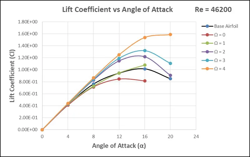
FIGURE 5.7: Comparison of Cl for the different spin ratio of the leading-edge cylinder
As can be seen from the figure leading-edge cylinder has very little or no effect
on the lift coefficient for a small angle of attack up around 8o. However, it shows
immense improvement in the lift coefficient for a higher angle of attack compared to
base airfoil for a high spin ratio. It is evident from the curve that at 4 spin ratios, the
lift coefficient at a higher angle of attack is increased by more than 200%. But to
achieve such a high spin ratio is practically very difficult as it rotates cylinder at
more than 4000 rpm. Hence, to have a balance between optimum performance
and practically achievable rotational speed of a cylinder is very important while
using a leading-edge cylinder for further application in wind turbines.
In a nutshell, it can be concluded from the use of a leading-edge cylinder is to
extend the lift curve hence substantially increasing the maximum lift coefficient
and delaying the stall effect.
Figure 5.8 shows the effect of the drag coefficient versus angle of attack for leading-edge
rotating geometry.
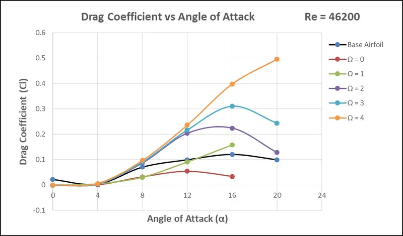
FIGURE 5.8: Comparison of Cd for the different spin ratio of leading-edge
cylinder
From the curve of a drag coefficient vs angle of attack, it is evident that drag
also increases with an increase in the spin ratio for a higher angle of attack. Although
the increase in drag coefficient is smaller when compared to the increase in lift coefficient
which has a positive influence on the lift to drag ratio. As the performance of an airfoil is
measured by the lift to drag ratio of an airfoil.
Hence, it is necessary to study how the overall lift to drag ratio of an airfoil
geometry behaves after the leading edge of an airfoil is replaced with a rotating cylinder
geometry as gave a clear indication of how and when such kind of model can
have real-life applications.
The figure below shows the curve of lift to drag ratio with the angle of attack at different
spin ratio.
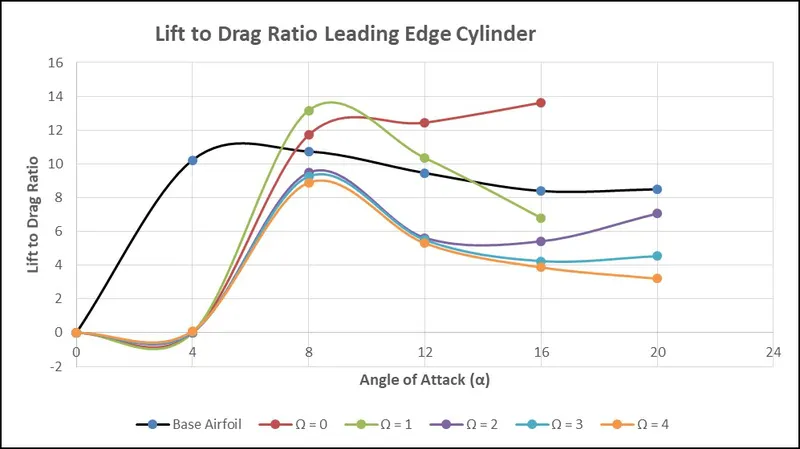
FIGURE 5.9: Comparison of lift to drag ratio for the different spin ratio
of leading-edge cylinder
From the above figure, one can conclude that leading-edge cylinder geometry
does not provide any significant improvement from the results of base airfoil lift
to drag ratio results. This suggests that there needs to be an improvement in the
model for a reduction in drag coefficient which can provide the results for further
application.
5.3 Analysis of Airfoil with Trailing Edge Rotating Cylinder
After testing the model with a leading-edge rotating cylinder, the next model is
tested with a trailing edge rotating cylinder. Unlike in the previous model in this
case geometry id drastically changes from the original airfoil. To accommodate
the cylinder on the trailing edge the airfoil chord is shortened by approximately 28%
which reduced the chord length from base airfoil to about 72%. Hence, the model
has a blunt trailing edge in the form of a cylinder. [1]
Figure 5.10 and 5.11 below shows the plot of lift coefficient and drag coefficient
respectively against the angle of attack for various spin ratio. As can be seen,
the trailing edge cylinder model behaves drastically opposite when compared
with the previous model. In this case, the model shows good results at a lower angle
of attack. Even at 0 angles of attack, the airfoil shows tremendous lift generation at
a higher speed of rotation of the cylinder.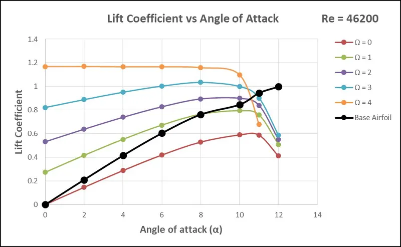
FIGURE 5.10: Comparison of lift coefficient for the different spin ratio
of leading-edge cylinder
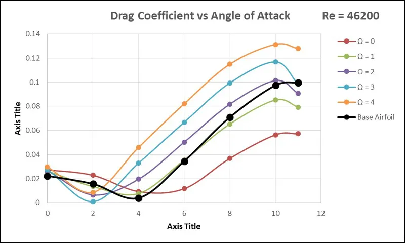
FIGURE 5.11: Comparison of the drag coefficient for the different spin ratio
of leading-edge cylinder
At a spin ratio of 0 hence in the absence of cylinder rotation, the model behaves
as base airfoil as pressure distribution over the airfoil is not change substantially.
With an increase in rotational speed of a cylinder, the suction on the upper surface
of an airfoil and compression over the lower surface of an airfoil increases
simultaneously.
This effect shows in the lift and drag curve represented ahead especially at a
high spin ratio and particularly at a lower angle of attack. Even at a higher angle of
attack, it shows improvement in lift coefficient when compared to the base airfoil
model even beyond the stall.
This is results in improving the lift performance for example at cylinder rotation
of W = 4 and angle of attack 4o, it shows 3 times increase in lift generation. "As
can be expected, the trailing edge cylinder essentially behaves as a flap shifting
the plots to the left. [1]"
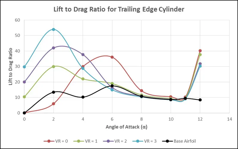
FIGURE 5.12: Comparison of lift to drag ratio for the different spin ratio
of trailing edge cylinder
Figure 5.12 shows the curve of lift to drag ratio against the angle of attack plotted
for various spin ratio.
Unlike the previous model which shows no improvement in lift to drag ratio,
this configuration shows improvement in lift to drag ratio for a smaller angle of
attack as can be evident from the previous explanation regarding the physics of a
model.
Hence, from a study of two simple modifications in a base airfoil, it is evident
that the performance of an airfoil can be improved by various configuration as
per the state of a need. Regardless of a geometrical modification used, the main
the objective of using the Magnus effect principle in wind turbine airfoil is to delay
the separation of flow over the top surface of an airfoil which in results improves
the overall performance.
5.4 Comparison of Results from Different Moving Frame Methods
Validation of any CFD results is based on its comparative study with Experimental
results of a similar study in a similar physical setup if such results are available.
It can also be compared with a different simulation approach within the CFD
tool. This section shows a comparative study of such an approach.
As stated above For further validation of the CFD tool, results extracted so far
have been achieved through the rotating wall and a steady-state approach needs to be
compared with another approach of simulation with sliding mesh and unsteady
or transient simulation method.
As the sliding mesh approach is a transient case, it is a time-consuming simulation
process. Hence here in this study, few results are compared from both
the study. The figure below shows the comparison of results from leading-edge
cylinder geometry for 2 different spin ratios. to cover all aspects one small and
one large spin ratios are selected which provide for good comparative study.
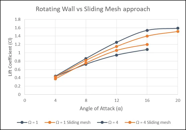
FIGURE 5.13: Comparison of simulation results from different moving
frame approach for leading-edge cylinder model
From figure 5.13 it is evident that the sliding mesh approach closely resembles
the rotating wall approach results. As can be seen for both curves of small and
large spin ratios, results from both approaches are very very much in agreement.
This close results further solidified the CFD model for the simulation of rotating
objects as well as the aerodynamic study of complex models.
Thereafter results for the trailing edge cylinder geometry are compared for
both the moving frame approach. In the previous case, a large angle of attacks
is chosen as a fact that leading-edge geometry mainly shows deviation from a base
airfoil at a larger angle of attack. While here small angle of attack range are selected
as trailing edge model shows deviation from a base airfoil at a smaller angle
of attacks.
The figure below shows the comparison of results between the moving wall
method and the sliding wall method for the trailing edge cylinder model.
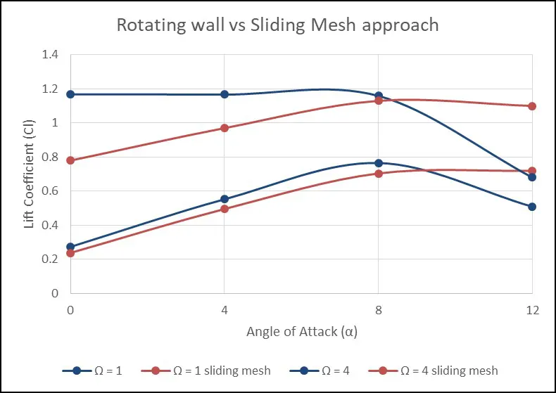
FIGURE 5.14: Comparison of simulation results from different moving
frame approach for trailing edge cylinder model
Figure 5.14, as can be it draws very interesting results. For the sliding
mesh approach results of 1 spin ratio have closely resembled until 8o angle of attack,
but thereafter at a higher angle of attack for rotating wall approach lift coefficient
does not drop suddenly as in the case with the rotating wall method.
Then after for 4 spin ratio results from rotating wall method are not that accurate
when compared to experimental results as at such a high cylinder rotation
rotating wall approach unable to provide for better simulation results. Whereas
with sliding mesh approach as can be seen from the curve provides good results
at a higher rotating speed of the cylinder.
The above study of comparison draws very interesting results, it shows that
the sliding mesh method is better at predicting results for high angle of attack
and high rotation of the cylinder. This indicates the stability of the CFD tool with
such an approach as in most cases with steady-state simulation it is hard to get
well converged results at such operating conditions.
5.5 Comparison of Simulation Results with Experimental Results
For validation of any simulated result, it is necessary to compare it with experimental
data. As experiments are performed over real physical conditions it
helps in validating the CFD model used for simulation. To compare with any
experimental results it is a must to keep in mind to provide similar physical conditions
and input data to closely resemble those results.
For comparison study in this thesis work experimental work of a Farzad Mokhtarian
[1], a mechanical engineer from Massachusetts Institute of Technology, USA;
is used as a base result. He performed experiments on "Fluid Dynamics of Airfoils
With Moving Surface Boundary-Layer Control".
The figure below shows the experimental results of a Lift coefficient against
the angle of attack for Leading-edge cylinder configuration over a Joukowsky airfoil.
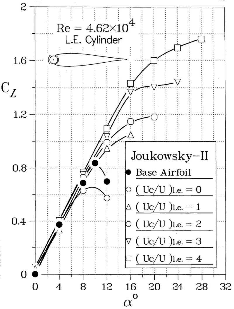
FIGURE 5.15: Effect of Leading-edge cylinder rotation on the lift and
stall characteristics of the Joukowsky model [1]
The experiment for this model is performed in a wind tunnel with pressure
tubes are attached all over the surface of an airfoil to collect data on pressure
distribution. The choice of such a small Reynolds number primarily driven by the
mechanical consideration of cylinder vibration at high rotational speed to achieve
such a high spin ratio.
As numerical data for experimental results are not presented in the research
paper, the online tool "WebPlotDigitizer" is used to generate values from the
above curve. Those values then plotted with simulation results generated. The
the figure below shows such a curve as a comparison of experimental results and
simulation results.
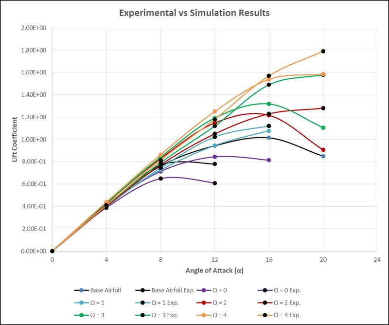
FIGURE 5.16: Comparison of simulation result with experimental
result for leading-edge cylinder model
In the above figure as can be seen curve with a "black" marking point represents
experimental results and the curve with "uniform color" represents simulation
results. From the above figure, it can be seen that simulation results closely resembles
experimental results.
However, there is a deviation in both results at a higher angle of attack. This
the deviation is primarily due to the fact that experiments are performed under real
physical conditions where effects of the far wall, temperature, and pressure resemble
better compared with simulation results using the CFD tool.
Such a variation is obvious when dealing with such complex problems as it
is near impossible to match all physical aspects of an experiment. overall simulation
results using leading-edge cylinder configuration is very much replicated
the experimental results and can be further used to study even complex configuration
for real-life practical application uses in wind turbines.
The figure below shows the experimental results of a Lift coefficient against
the angle of attack for Trailing edge cylinder configuration over a Joukowsky
airfoil.
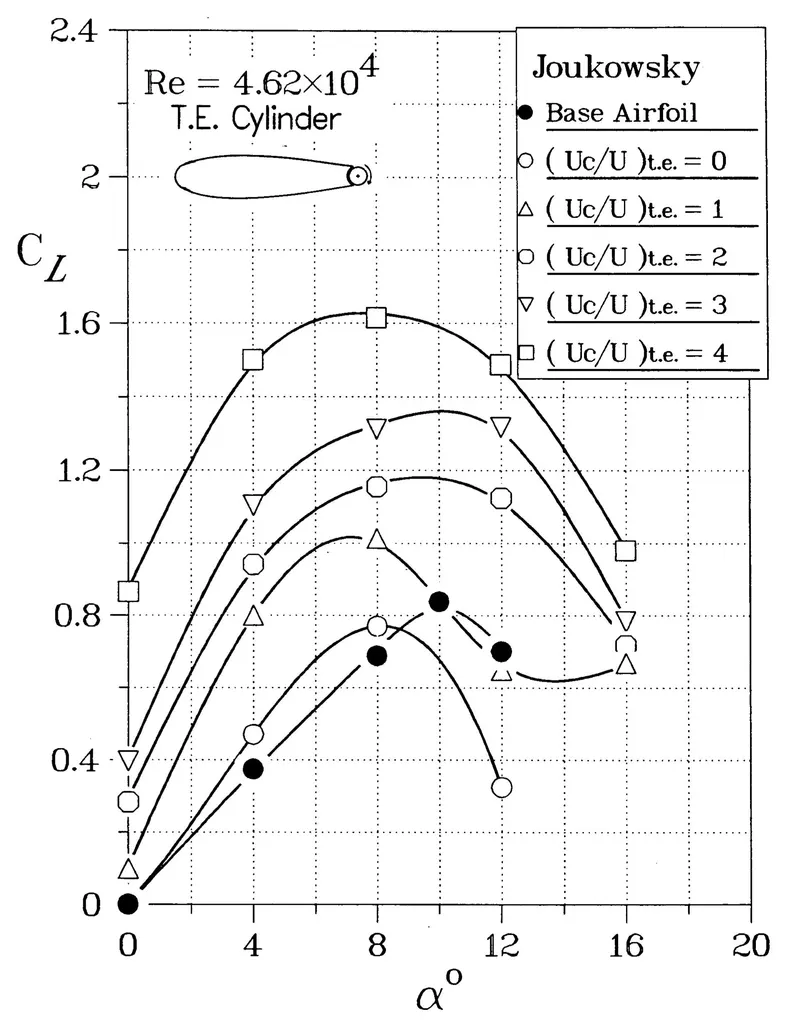
FIGURE 5.17: Effect of Trailing-edge cylinder rotation on the lift and
stall characteristics of the Joukowsky model [1]
From the above figure, it is evident that unlike leading-edge geometry which
increases lift beyond the stall angle and delay the stall with an increase in rotational
speed, trailing edge cylinder configuration increase the lift before the stall
angle.
After extracting the numerical values from the plot above it is plotted with
simulated results for comparison. Figure 5.16 shows the comparison curve for
experimental and simulation results. Unlike previous comparisons in the case of
a leading-edge cylinder, these results show much deviation from the experimental
results especially at a higher angle of attack. A turbulent model is unable to
converge results at such a high angle of attack.
However, it can be seen from both the results that trailing edge cylinder configuration
shows a high increment in lift coefficient up to 8o angle of attack. Results
for both experimental and simulation are showing stall at 8o angle of attack. It is
a good resemblance as far as using such configurations is a concern. Both the
results are showing good competency from 2o to 8o angle of attack.
Such a variation is obvious when dealing with such complex problems as it is
near impossible to match all physical aspects of an experiment as discussed for
the previous configuration. Overall simulation results using trailing edge cylinder
the configuration is very much replicated the experimental results and can be
further used to study even complex configuration for real-life practical application
uses in wind turbines.
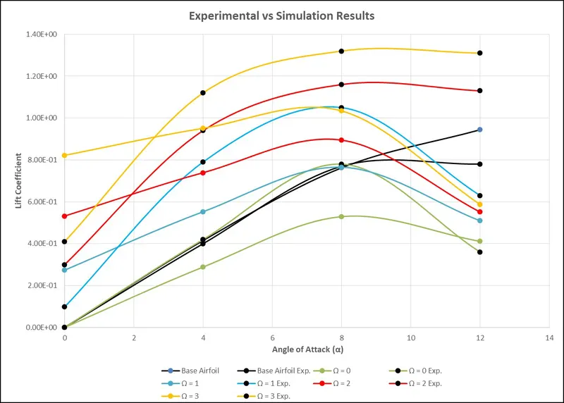
FIGURE 5.18: Comparison of simulation result with experimental
result for trailing edge cylinder model
Relative error study between different simulation method approach with
experimental results :
To compare quantitatively how much different method affects the output results
here presented a comparative study of errors or deviation of results from
experimental results.
The histogram in figure 5.19 shows an error in percentage between moving wall
method results and sliding mesh approach results from experimental values for
different cases for the leading-edge cylinder model.
As can be seen from the error plot of the leading-edge cylinder model for smaller
the angle of attack sliding mesh approach is better compared to the rotating wall method
as it gives relatively closed results with experimental results whereas for higher
angles this deviation is increasing as the CFD tool are not comparatively good at
the higher angle of attacks.
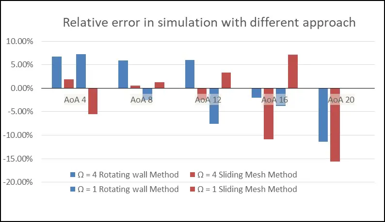
FIGURE 5.19: Comparison of relative error with different simulation
approach for leading-edge cylinder model
The histogram in figure 5.20 shows an error in percentage between moving wall
method results and sliding mesh approach results from experimental values for
different cases for the trailing edge cylinder model.
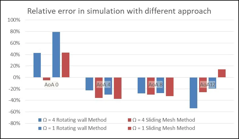
FIGURE 5.20: Comparison of relative error with different simulation
approach for trailing edge cylinder model
As can be seen from the above error plot it is visible that the sliding mesh approach
closely resembles experimental results compared with the rotating wall
method. However, the relative error in the trailing edge cylinder case is slightly
in a higher range of 40% to 60% when compared with the leading-edge model.
This is due to the fact that the leading edge cylinder model is not much complex
in design and it closely matches the base airfoil shape whereas the trailing
edge model is a slightly complexly design model with a blunt end which affects the
simulation results.
5.6 Effect on Coefficient of Pressure (Cp) due to cylinder rotation
The coefficient of pressure (Cp) is an important parameter to study after simulating
any airfoil model. It helps in how pressure is varying over an airfoil surface
which in turn results in force generation. This section shows how various operating
conditions changes pressure over the airfoil surface.
Cp variation in leading-edge cylinder model :
Below presented are few curves to see how Cp varies due to change in rotational
speed of a cylinder for the constant angle of attack.
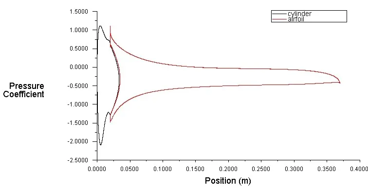
FIGURE 5.21: Cp curve for leading edge model at a = 16o for W = 0
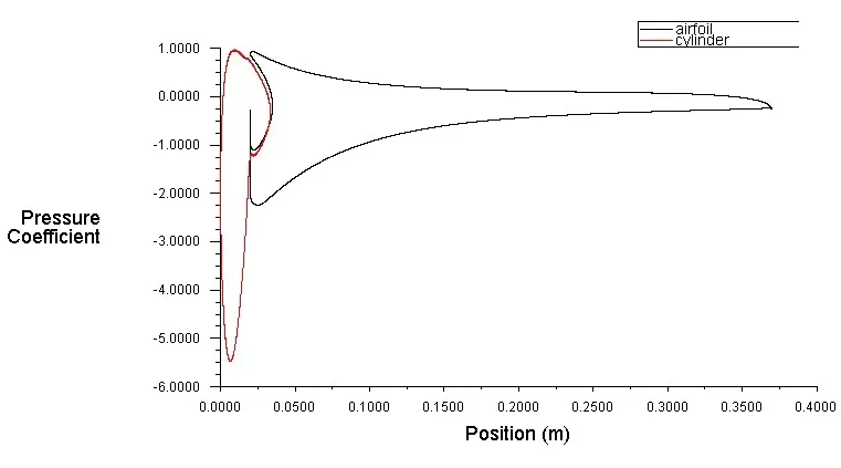
FIGURE 5.22: Cp curve for leading edge model at a = 16o for W = 2
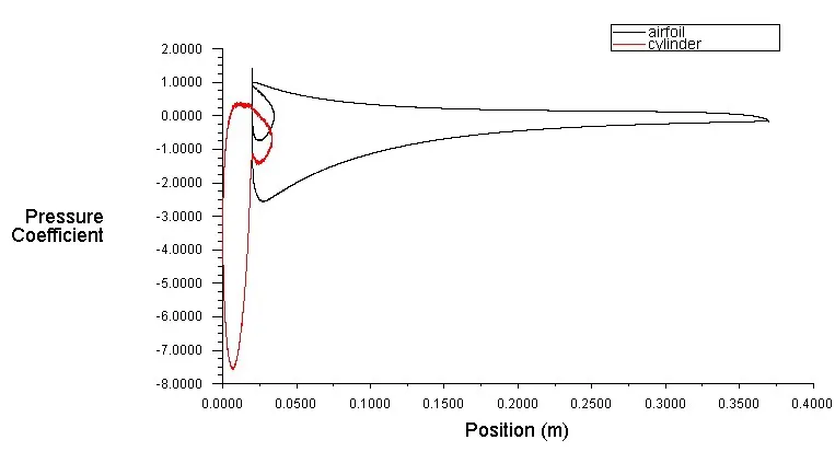
FIGURE 5.23: Cp curve for leading edge model at a = 16o for W = 4
From the above set of curves, it can be seen that with an increase in rotational
speed of cylinder negative pressure increase below the surface of the cylinder.
This pressure drop eventually increasing lift in the airfoil. Hence it is evident
that for the constant angle of attack, the lift can be an increase in airfoil by changing the
speed of a cylinder rotation.
Cp variation in trailing edge cylinder model :
The trailing edge cylinder model behaves differently in terms of Cp compared
to the previous model. This case model does not have a sharp trailing edge
due to the presence of a cylinder. Due to this blunt trailing edge rotation of cylinder has
a more positive effect towards increment in the lift. Below is the plot of a variation
of Cp along the model surface for the constant angle of attack 8o with a different Spin
ratio.
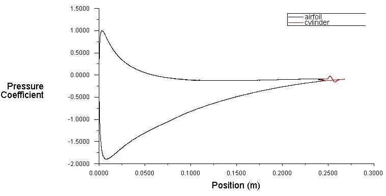
FIGURE 5.24: Cp curve for trailing edge model at a = 8o for W = 0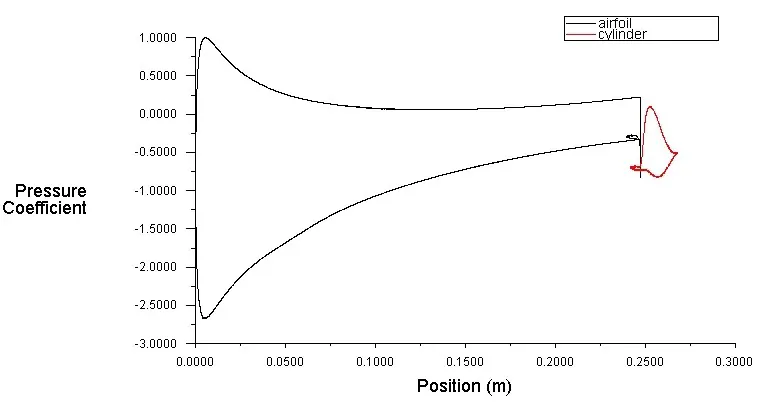
FIGURE 5.25: Cp curve for trailing edge model at a = 8o for W = 2
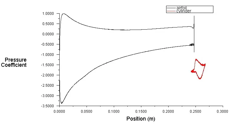
FIGURE 5.26: Cp curve for trailing edge model at a = 8o for W = 4
As can be seen from the above plots of a Cp for the trailing edge cylinder model,
with an increase in rotational speed of a cylinder low pressure is generated below
the cylinder surface and also flow remains attached to the airfoil at the trailing
edge. Flow attachment creates a delay in separation at the trailing edge which eventually
generates a high lift in the model.
5.7 Post-processing of Simulation Result
Results of simulation help in determining the validity of a model and tool but it
does not give a clear picture of the actual physics behind the process. Post-processing
is an essential part of any CFD simulation as it gives an understanding of how the
fluid flow is behaving in a particular physical state hence give a clear idea about
the nature of flow and when it is changing behavior at any particular instant
during the flow.
After performing all the required simulations for the comparison of different
results, it is necessary to visualize the actual flow pattern to summarise the behavior
of fluid in this case for various angles of attack and at various velocity ratios.
This section represents the results of velocity and pressure contour for both
leading edge and trailing edge cylinder model. Few sample results are presented
for the particular operating condition to have a better comparative study
of changes in physical quantity with changes in input conditions.
5.7.1 Velocity Contour of Leading Edge (LE) Cylinder Geometry
Velocity contour represents average cross-sectional flow velocity at every point
in a domain. Velocity contour helps in better flow visualization with a change in
operating conditions such as the angle of attack or cylinder speed, according to this
study.
Figures 5.27 to 5.30 represents the pattern of velocity around the leading edge
cylinder model, few sample post-processing results show below at W = 1 for
the varying angle of attack to see how velocity contour changes with change in angle
of attack for constant spin ratio.
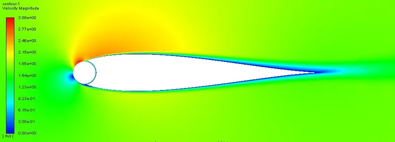
FIGURE 5.27: Velocity Contour for LEC model at W = 1 and a = 4o
As can be seen from figure 5.27 with rotation in a cylinder in a clockwise direction,
flow helps with the momentum of cylinder rotation and rapidly flew past
the upper surface of the airfoil. Velocity on the lower surface is relatively small
for a smaller angle of attack. As can be seen in figure 5.28 and 5.29 these changes
are increasing with an increase in the angle of attack. This difference in velocities on
both sides cause lift force generation in the airfoil.
As can be seen from figure 5.28 onward with an increase in the angle of attack
velocity is an increase on the upper surface of the airfoil blade and simultaneously
decrease on the lower surface of a blade. Hence, an increase in the angle of attack, the
the difference in velocities between both surfaces increases which helps in generates
more lift.
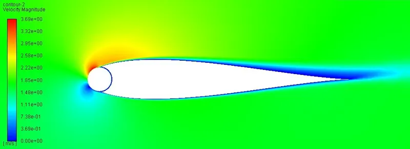
FIGURE 5.28: Velocity Contour for LEC model at W = 1 and a = 8o
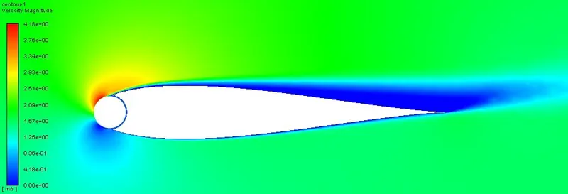
FIGURE 5.29: Velocity Contour for LEC model at W = 1 and a = 12o
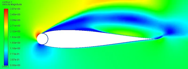
FIGURE 5.30: Velocity Contour for LEC model at W = 1 and a = 16o
The previous case shows how the angle of attack changes flow velocity distribution
in a leading-edge cylinder at a constant speed of the cylinder. Thereafter it is
interesting to see how cylinder speed affects the velocity distribution around the
airfoil by keeping a constant angle of attack. Figures below show the results of the velocity
contour by keeping the constant angle of attack and changing the spin ratio to see the
effect of the rotational speed of the cylinder on the flow pattern.
FIGURE 5.31: Velocity Contour for LEC model at W = 1 and a = 12o
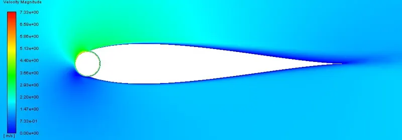
FIGURE 5.32: Velocity Contour for LEC model at W = 4 and a = 12o
From the above 2 contours, it can be visualized that with an increase in rotational
speed of a cylinder even at a constant angle of attack, velocity increases dramatically
on the top surface of the airfoil blade as the flow remains attached to the high-speed
cylinder as can be seen from the values of velocities on both figures and it also increases
negative pressure on the lower surface of the airfoil blade. This phenomenon
known as the Magnus effect, helps in generating lifting force on the cylinder and
simultaneously whole airfoil model experiences an increment in lift force due to
cylinder rotation.
Although there is a critical cylinder speed beyond which it is not possible to
increase lift as much high speed has a negative effect on flow behavior and also
in practice, it is not feasible to attain such a high cylinder speed.
5.7.2 Pressure Contour of Leading Edge (LE) Cylinder Geometry
After visualizing velocity contour for the leading edge cylinder model, here presented
contour of pressure to see how pressure is changing with different operating
conditions due to the presence of cylinder. Below figures represent the
pressure contour of a model for constant W = 1 and varying angle of attack.
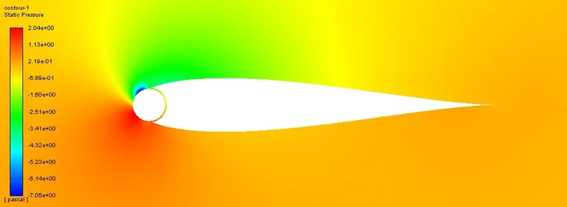
FIGURE 5.33: Pressure Contour for LEC model at W = 1 and a = 8o
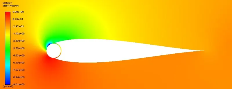
FIGURE 5.34: Pressure Contour for LEC model at W = 1 and a = 12o
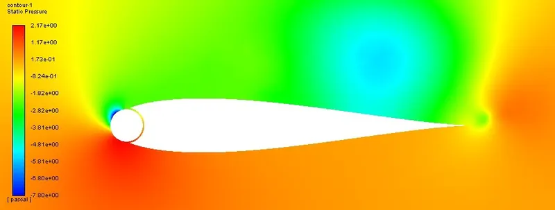
FIGURE 5.35: Pressure Contour for LEC model at W = 1 and a = 16o
Figure 5.33 to 5.35 shows the pressure distribution contour around leading-edge
cylinder model. From the above pressure contour, it can be seen how changing
in the angle of attack create high pressure below the cylinder and airfoil body and
low pressure on the upper surface of the model, these pressure difference results
in lift generation in a model.
The below figures show few results of pressure contour by keeping a constant angle
of attack and changing the spin ratio to see the effect of the rotational speed of the cylinder
on the flow patterns.
FIGURE 5.36: Pressure Contour for LEC model at W = 1 and a = 12o
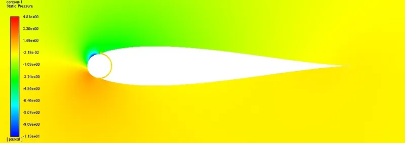
FIGURE 5.37: Pressure Contour for LEC model at W = 4 and a = 12o
As can be depicted from the figure above pressure is increased on the lower
surface of an airfoil from 2.09 pascal to 4.81 pascals with a change in spin ratio
from 1 to 4. Also, pressure on the upper surface decrease from -9.61 pascal to
-11.3 with an increase in spin ratio.
This pressure difference is results in a dramatic increase in lift coefficient in
airfoil even at a constant angle of attack.
5.7.3 Velocity Contour of Trailing Edge (TE) Cylinder Geometry
To see the pattern of velocity around the trailing edge cylinder model, a few samples
post-processing results show below at W = 1 for various angles of attack to see
how velocity contour changes with change in the angle of attack for a constant spin
ratio.
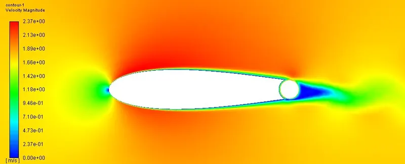
FIGURE 5.38: Velocity Contour for TEC model at W = 1 and a = 0o
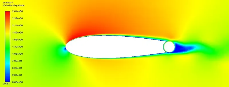
FIGURE 5.39: Velocity Contour for TEC model at W = 1 and a = 4o
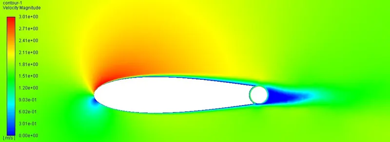
FIGURE 5.40: Velocity Contour for TEC model at W = 1 and a = 8o
Figure 5.38 to 5.40 shows the velocity contours of a model, it can be seen how
changing in the angle of attack makes flow separation delay on the top surface of an
airfoil which in results increases the lift value and decrease the drag.
Thereafter it is important to see the effect of spin ratio or cylinder rotation
speed on velocity distribution in the trailing edge cylinder model by keeping a constant
angle of attack. Below 2 figures shows the velocity contour at 12o angle of
attack for W = 1 and W = 4.
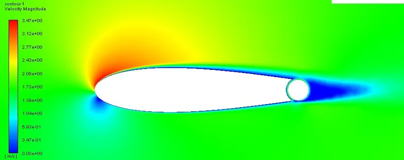
FIGURE 5.41: Velocity Contour for TEC model at W = 1 and a = 12o
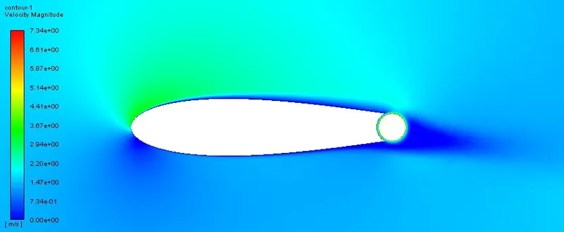
FIGURE 5.42: Velocity Contour for TEC model at W = 4 and a = 12o
From the above 2 velocity contours, it is clearly visible how changes in the speed of
rotation of cylinder increases maximum velocity on the top surface of an airfoil from
3.47 m/s to 7.34 m/s. Cylinder rotation also helps in the attached flow over the
the upper edge of an airfoil and delaying separation at the trailing edge. This delay in
separation increase with cylinder speed as flow unable to separate quickly due to
high speed in the cylinder and blunt trailing edge instead of sharp one, which further
helps in increment in the lift.
5.7.4 Pressure Contour of Trailing Edge (TE) Cylinder Geometry
To see how pressure changes in the trailing edge cylinder model with the various setting,
the spin ratio is set at W = 1 and by varying angle of attack pressure contour is
generated from simulation results. Below presented are such a set of contours
to analyze how different angles of attack affect the pressure distribution in the
model.
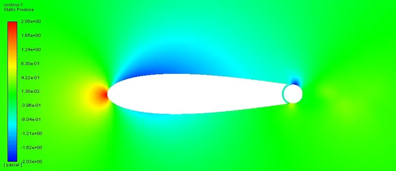
FIGURE 5.43: Pressure Contour for TEC model at W = 1 and a = 0o
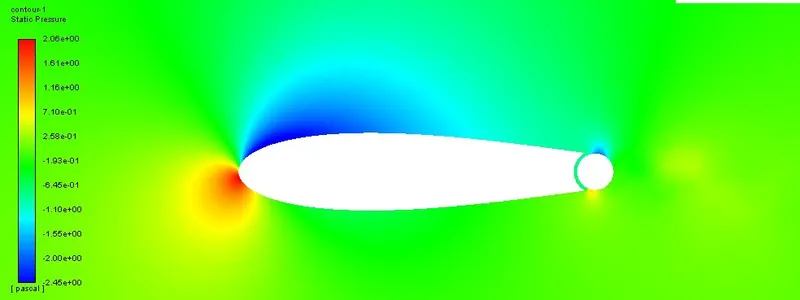
FIGURE 5.44: Pressure Contour for TEC model at W = 1 and a = 4o
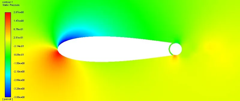
FIGURE 5.45: Pressure Contour for TEC model at W = 1 and a = 8o
From the above pressure contours, it can be seen how changes in the angle of
attack increase negative pressure below the cylinder and airfoil body. Figure 5.43
shows that even with no angle of attack airfoil generates lift due to the rotation
of the cylinder which generates velocity and pressure difference between the two
surfaces of the airfoil model. As can be seen from the subsequent figures this
difference between pressure is increasing with an increase in the angle of attack.
The below figures show few results of pressure contour by keeping a constant
angle of attack and changing the spin ratio to see the effect of the rotational speed of
the cylinder on the flow pattern.
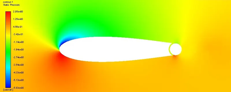
FIGURE 5.46: Pressure Contour for TEC model at W = 1 and a = 12o
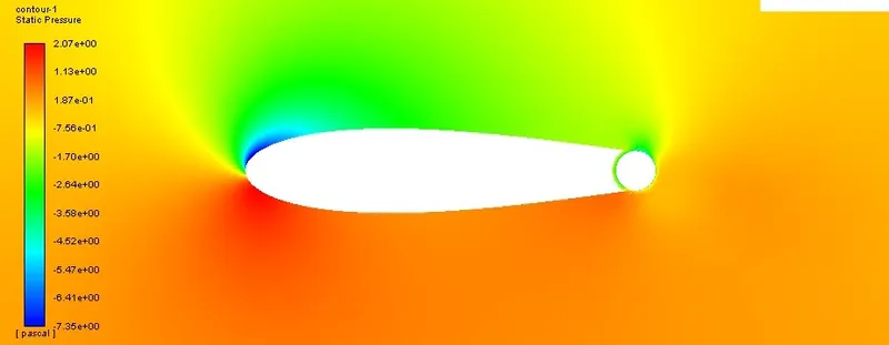
FIGURE 5.47: Pressure Contour for TEC model at W = 4 and a = 12o
From figure 5.46 and 5.47, it can be seen that negative pressure is increased
highly with an increase in cylinder rotation speed. with a spin ratio of 1, negative
pressure on the top surface is around -5.93 pascal which decreases to -7.35 pascal
with an increase in spin ratio up to 4. Whereas pressure on the lower part of
the surface remains almost constant as can be seen from the values in the figures.
However, due to an increase in pressure difference, which is mainly helpful for lift
increment, it can be seen that even at a constant angle of attack, airfoil generates
more lift with an increase in cylinder rotation speed up to optimum achievable
value.
Chapter 6 Conclusion
The study of modified symmetric Joukowsky airfoil with a rotating cylinder attached
to it at leading and trailing edge is simulated at appropriate physical conditions
with well modeled and meshed geometries. This simulated result yields
quite an interesting aspect regarding the effect of the Magnus phenomenon on airfoil
performance. Below listed are a few important conclusions and remarks from the
obtain simulated results.
- Modified Joukowsky airfoil with a leading-edge cylinder results in increased
suction over the nose. This propagation of an increase in the negative pressure
coefficient leads to a delay in flow separation at a higher angle of attack. - The effectiveness of a leading-edge rotating cylinder also depends on how
smoothly flow transition from cylinder surface to airfoil surface. From the
results of the comparison between different geometries with varying gap
sizes, it is concluded that the gap of more than 2mm reduces the effectiveness
of the cylinder for the airfoil of 370mm chord length. - With an increase in cylinder rotation speed more momentum is injected into
the boundary layer which eventually delays the separation of flow from the
top surface and result in a higher lift coefficient. However, there is some
the critical rotational speed of cylinder beyond which it has relatively less effectiveness
in lift increment. - Leading-edge cylinder modification does not change the overall configuration
of an airfoil, which means it has a round leading edge and sharp
trailing edge. The use of the leading edge cylinder extends the lift curve
beyond the stall angle with an almost similar slope of the curve to that of the base
airfoil. Hence, a leading-edge cylinder extends the stall angle as well as the
maximum lift coefficient. - As stated in the above points lift and stall characteristics are significantly
improved with a leading-edge rotating cylinder. To cite an example, the maximum
lift coefficient measured with W = 4 is 1.8 for 20o angle of attack
which is almost 2 times the lift coefficient of a base airfoil. - Unlike the leading-edge cylinder model, the trailing edge cylinder model
behaves differently as it has slightly varying geometry compared to the base
airfoil. To accommodate the rotating cylinder at the trailing edge, the tail of
the modified geometry is blunt in shape which changes the physics of flow
separation. - The high rotating speed of the trailing edge cylinder results in an
increase in suction over the upper surface of the airfoil. which delays the
trailing edge flow separation. Hence, it results in a dramatic increment in
the lift coefficient even at 0o angle of attack. - The leading-edge cylinder extends the lift curve beyond the stall angle whereas
the trailing edge cylinder increases the lift before the stall angle. For this
model stall angle almost remains the same for different cylinder rotation
but lift shows a significant increase before the stall angle is reached. - It can also be derived from the study of both the model with sliding mesh
an approach that both methods are good at resembling experimental results.
However, it is interesting to see that at a higher angle of attack, sliding mesh
the approach gives lower relative error due to the fact that at such a high angle of
attack and with rotating and stationary zones are placed adjacent to each
other, unsteady simulation is better to approach as covers all the aspect in such
complex models.
Bibliography
[1] Farzad Mokhtarian. “Fluid Dynamics of Airfoilswith Moving Surface Boundary
Layer Control”. In: The University of British Columbia, The Faculties of grade
studies, Department of Mechanical Engineering(1988), pp. 1–2.
[2] J. Seifert. “A review of the Magnus effect in aeronautics”. In: The University
of British Columbia, The Faculties of grade studies, Department of Mechanical Engineering(
1988), pp. 1–2.
[3] ŁOPACIUK P. “Wizualizacja efektu Magnusa z wykorzystaniem bibliotek i
OpenGL.”In:Diploma Thesis, Chełm(2007).
[4] “Lift on rotating cylinders”.In: NASA Glenn Research Center (2010-11-
09.Retrieved 2013-11-07).
[5] Marchaj "Aero Hydrodynamics of Sailing," Dodd, Mead pp. 172-198. (Ref. 23).
[6] T. Hanyuand, N. Murakami, H. Hasegawa, and M. Nakamura. “The Mechanism
of Flow Field around a Rotating Cylinder with Fins for High Performance
MagnusWind Turbine”.In: Journal of Energy and Power Engineering, Vol. 10, No.1
(2016), pp. 23–31.
[7] Hiroaki Hasegawa Masaya Ueki and Yuya Ikezawa. “Lift Enhancement of
a Rotating Cylinder for Magnus Wind Turbine”.In: Grand Renewable energy
2018 Proceedings, Utsunomiya University(2018). DOI:[email protected].
ac.jp.
[8] Christophe Sibuet Watters Jonathon Sumner.“CFD in Wind Energy: The-
Virtual, Multiscale Wind Tunnel”. In:Energies 2010 (17 May 2010), 55:17–45.
doi:10.3390/en3050989.
[9] L Prandtl. “Application of the Magnus Effect to the wind Propulsion of Ships
(Translation)”. In: AEC Report NACA TM 367 (National Aeronautics and Space
Administration, Washington, D.C.(1924).
[10] W. W. Wood. “Boundary Layers Whose Streamlines are Closed”. In: Aeronautical
Research Laboratories, Fishermans Bend, Melbourne, Australia. (1956).
[11] M. B. Glauert. “The Flow Past a Rapidly Rotating Circular Cylinder”. In:
Royal Society of London Proceedings Series A.242 (1957), pp. 108–115.
[12] D. C. Thoman and A. A. Szewczyk. “Numerical Solutions of Time-Dependent
Two-Dimensional Flow of a Viscous, In-compressible Fluid Over
Stationery and Rotating Cylinders”. In: Department of Mechanical Engineering,
University of Notre Dame (Notre Dame, Indiana)Report TR66-14 (1957).
[13] Howard Leon Power Jr. “Boundary layer contribution to the Magnus effect
on a spinning cylinder at low angles of attack”. In: Iowa State University Engineering,
aeronautical(1971), pp. 2–3.
[14] Vincent R. Den Hertog. “Moving surface boundary layer control with application
to autonomous underwater vehicles”. In: The Faculties of Graduate
Studies, Department of Mechanical Engineering, The University of British Columbia,
Vancouver, Canada(1999), pp. 3–4.
[15] L. Prandtl. “Zur berechnung der grenzschichten.” In: ZAMM-Journal of
Applied Mathematics and Mechanics/Zeitschrift für Angewandte Mathematik und
Mechanik 18.1(1938), pp. 77–82
[16] Klaus Gersten Hermann Schlichting (Deceased). “Boundary-Layer Theory”.
In: Institute of fluid mechanics, Technische Universität Braunschweig, Deutschland.(
1955), pp. 38–39.DOI:10.1007/978-3-662-52919-5.
[17] Epifano V. M. “N. E. Bauman Moscow State Technical University,
Moscow”.In: National Committee for Heat and Mass Transfer, Russian Academy
of Sciences, Russia DOI:10.1615/AtoZ.b.boundary-layer.
[18] Sazo Knez. “Airfoil boundary layer”. In: Faculty of mathematics and physics,
University of Ljubljana (2005), p.7. DOI:http://www.f1.ijs.si/rudi/sola/drugiseminar.
pdf.
[19] https://www.perfectedflight.com/the-truth-about-induced-drag.
[20] https://www.grc.nasa.gov/www/k-12/airplane/cp.html.
[21] L. J. Clancy. “Aerodynamics”. In: New York: JohnWiley & Sons, Sections 4.15 &
5.4(1975).
[22] Ira H. Abbott and Albert E Doenhoff. “Theory of Wing Sections”. In: Dover
publications, Inc. New York, Section 1.2(1958).
[23] Barnes W. McCormick. “Aerodynamics, Aeronautics, and Flight Mechanics”.
In: John Wiley & Sons, Inc., New York(1979),p. 24.
[24] Abdelrady Okasha Elnady Mohamed A. Fouad Kandil. “Performance of
GOE-387 Airfoil Using CFD”. In: Mechatronics Department, Faculty of Engineering,
The University of Egypt, International Journal of Aerospace Sciences 20175(1) (1979),
pp. 1–7. DOI: 10.5923/j.aerospace.20170501.01
[25] On the Application of Rotating Cylinders to Micro Air Vehicles By Carmine Badalamenti
School of Engineering and Mathematical Sciences, City University London,
Northampton Square, London, EC1V 0HB, July 2010.
[26] Tracie Barber/Eddie Leonardi, In CFD Modeling of Wind Tunnel, Flow over a
Rotating Cylinder John Middendorf, Computation Fluid Dynamics, May 30, 2003
[27] https://mixing-solution.com/2012/07/31/mrf-versus-sliding-mesh.
[28] http://mathfaculty.fullerton.edu/mathews/c2003/JoukowskiTransMod.html
[29] DR. FRIEDRICH WILHELM RIEGELS, Aerofoil sections results from wind tunnel
investigations(1961), Butterworths, London.
[30] Essential MATLAB for Engineers and Scientists (2013) PART 2-
Applications, CHAPTER 14 - Introduction to Numerical Methods.
https://apprize.info/software/matlab/14.html.