Challenge on Combustion

Aim: Simulation of Combustion using ANSYS Fluent

Objective:

Part I

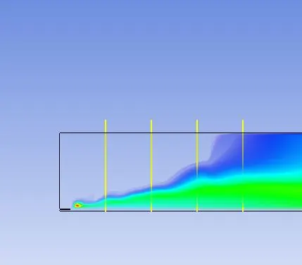
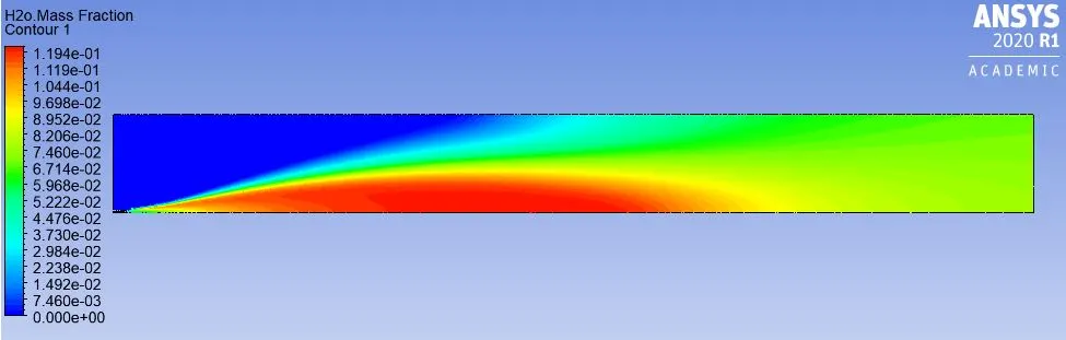
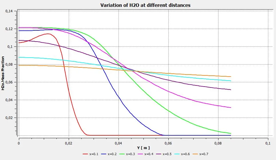
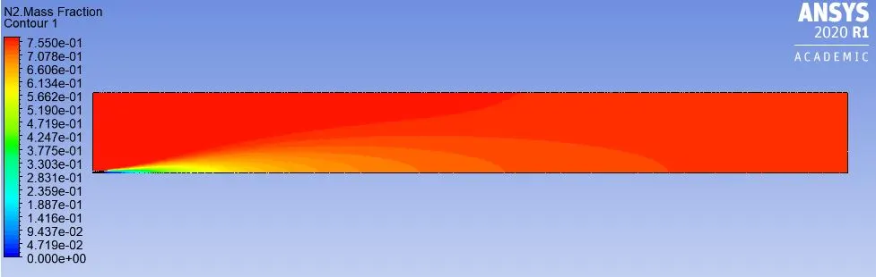
Perform a combustion simulation on the combustor model and plot the variation of the mass fraction of the different species’ in the simulation using line probes at different locations of the combustor as shown in Fig. You need to plot for CO2, H2O, CH4, N2, O2, NOx emissions & Soot formation.

Part II

As you must have observed from the above simulation, the NOx and Soot are getting formed at the outlet of the combustor. Such formation has harmful effects on the environment and humans. The stringent government norms also demand the least formation of Nox and soot and to satisfy those requirements, you need to check the effect of adding the water to the fuel.

In this part, you need to add the water content in the fuel from 5% to 30% by mole and observe the effect of it on the results. It is necessary to provide line plots and contours to prove your claim.

Theory of Combustion:

It is a high-temperature exothermic reaction (redox) between a fuel (reductant ) and an oxidant or the oxidizer to release a large amount of chemically bound energy. A flame is a characteristic indicator of the combustion reaction.lt is a sequence of elementary radical reactions. Solid fuels undergo endothermic pyrolysis to generate gaseous fuel whose combustion supplies the heat required to produce more of such gaseous fuel products. The formation of these products is very complex and many different species such as H, 0, OH, CH3, CH4 are formed in the process. Besides Carbon dioxide and water a large no. of pollutants like Nitrous oxide, Carbon mono oxide, and soot particles are formed. A simple example can be seen in the combustion of Hydrogen and Oxygen into water vapor, a reaction generally used to fuel the rocket engines. The reaction releases 250KJ/mol of heat and reduces the enthalpy at constant temperature and pressure.

Types of combustion models:

1. Based on combustion:

Non-Premixed Combustion: In non -premixed combustion fuel and oxidizer enter the reaction zone in separate streams and are not mixed before combustion.Whereas in premixed combustion reactants are mixed with the oxidizer at the molecular level before burning or combustion takes place.

• Examples: Diesel Internal Combustion Engines and pool fires. This is applied only for turbulent flows by using a pressure-based solver.

a) Premixed Combustion: This type of combustion happens when fuel and oxidizer are mixed before burning. They are mixed at the molecular level. Here the flame front propagates into the unburnt reactions as the combustion takes place.

• Examples: Gas Leak combustion explosions, premixed gas-turbine combustors.

Pressure based solver is used and is applicable for turbulent flows and subsonic flows. This type of flames called detonations or deflagrations or explosions, where the combustible mixture is ignited by a heat source behind a shock wave. The Premixed combustion model cannot be used along with the NOx pollutant model and soot model turned on, whereas the partially premixed model can be used along with the pollutant model turned on. Only inert particles can be used for simulation by the premixed combustion model, not the discrete phase particles.

b) Partially premixed combustion:

Here fuel and oxidizer are primarily mixed before combustion. They are the premixed flames with non-uniform fuel-oxidizer mixtures. It is a model combustion process intended to be used in Internal combustion engines of motorized vehicles and other automobiles. Its high specific power, high fuel efficiency, and low exhaust pollution made it a promising technology. These premixed flames involve premixed jets discharging into the atmosphere, lean premixed combustors with cooling air jets, or diffusion pilot flames. In order to compute the concentrations of individual species, a partially premixed combustion model is used. This is applicable for turbulent flows by the use of a pressure-based solver.

2. Based on Phases:

a) Fluid phase: Combustion happens when fuel is in the fluid phase.

b) Volumetric phase/gas phase: It is for gas-phase reactions. The reaction rates are defined on a volumetric basis.

c) Wall surface: For gas-phase reactions, the reaction rate is defined on a volumetric basis. Here combustion happens on a wall or boundary. For surface reactions, the rate of adsorption and desorption is governed by both chemical kinetics and diffusion process. When the volumetric is enabled, wall surface reactions create sources and sinks of species in the gas phase enabling the calc of wall surface reaction kinetics. They are also applied to the reacting surface.

d) Particle surface: Combustion happens over surfaces involving multi-phase particle surface reaction mechanism. This is applied by using the volumetric turned on.

MODELLING AND MESHING

Geometry:

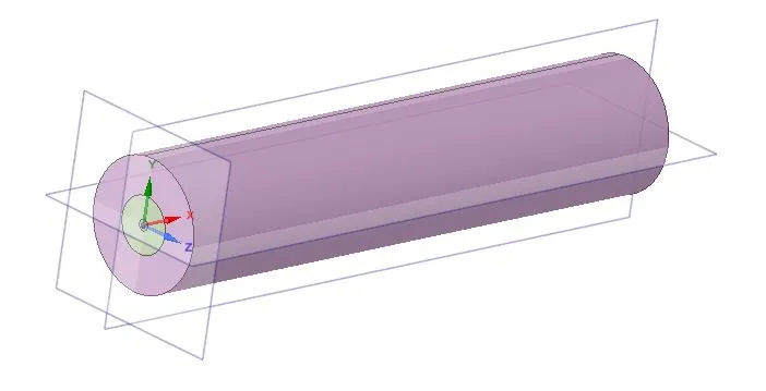
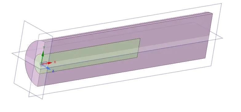
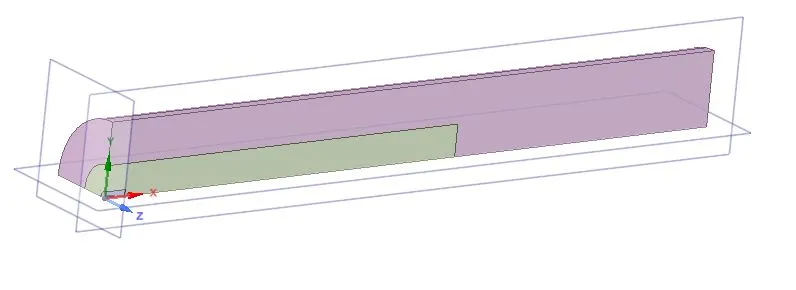
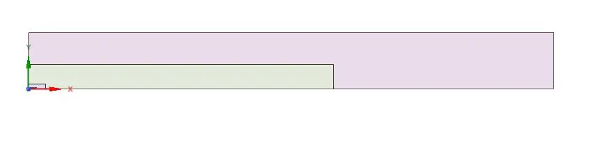
Only 1/4th part of the model is used for analysis. A body split tool is used for splitting bodies. The 2D front face is used for analysis by a copy-paste tool.

The process of 3d Model to 2D Model is shown in the below figures step by step.

2D geometry for Analysis:

Meshing:

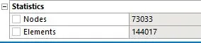
The next step after generating a 2D model is to mesh a model for further simulation.

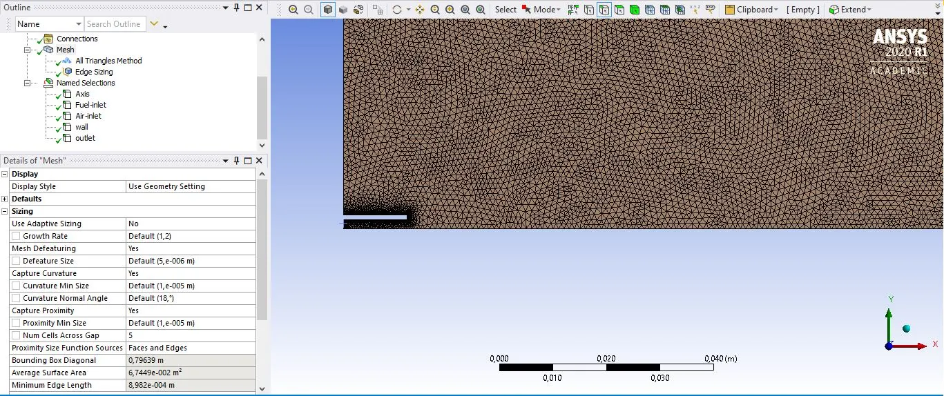
As can be seen from the geometry, greater care needs to be taken at the fuel inlet section as there are narrow gaps in that section.

Named Selections:

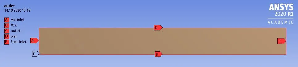
After generating optimum fine meshing, the next step is to give name selection to the boundaries for specifying physical properties at particular boundaries. The Name Selections in the model are as shown in the figure below.

NUMERICAL AND BOUNDARY CONDITION SETUP IN FLUENT:

After a discretizing a model with optimum meshing, the next step is to give physical setup and boundary conditions for the required cases, to run the simulation, and generates results of the fuel and air mixing study.

The inputs for the fluent setup is as stated below.

• Solver- Pressure based
• Steady-state Simulation
• 2D-Planar Axisymmetric
• Viscous Turbulence model- K epsilon -> Standard -> Scalable wall functions
• Species Model Turned ON

Species Model :

Species:

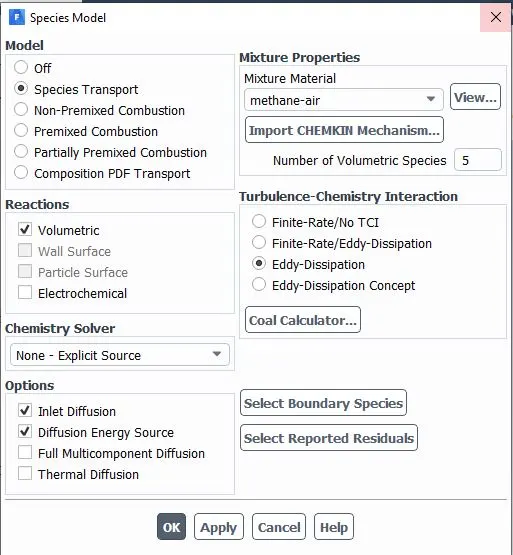
The Species Model dialog box allows you to set parameters related to the calculation of species transport and combustion.

Species Transport - enables the calculation of multi-species transport (either non-reacting or reacting, depending on the selection for Reactions).

Reactions - contains options related to the modeling of reacting flow.

Volumetric - enables the calculation of reacting flow using the finite-rate formulation.

Inlet Diffusion - includes the diffusion flux of species at the inlet.

Diffusion Energy Source - includes the effect of enthalpy transport due to species diffusion in the energy equation.

Mixture material - Methane-air 2 step is used as it allows the addition of water in fuel or air

NOX and Soot model is turned ON:

1) NOx Model

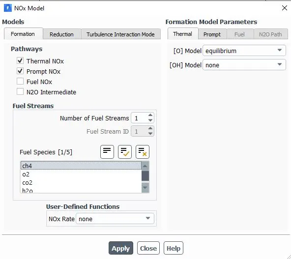
Mainly consists of Nitric oxide (NO), Nitrogen peroxide (NO2), and Nitrous oxide (N20) to a smaller extent Thermal, Prompt, Fuel, and N20 intermediate mechanisms are available.

Thermal NOx - It is formed when nitrogen and oxygen in the combustion air combine with one another at the high temperatures in a flame.

Prompt NOx - Forms from the rapid reaction of atmospheric nitrogen with hydrocarbon radicals.

Fuel NOx - It is formed by the reaction of nitrogen bound in the fuel with oxygen in the combustion air. It is rarely a problem with gaseous fuels.

In our case, we will activate Thermal and prompt NOx, as there is no nitrogen in input fuel as is Methane CH4.

2) Soot Model

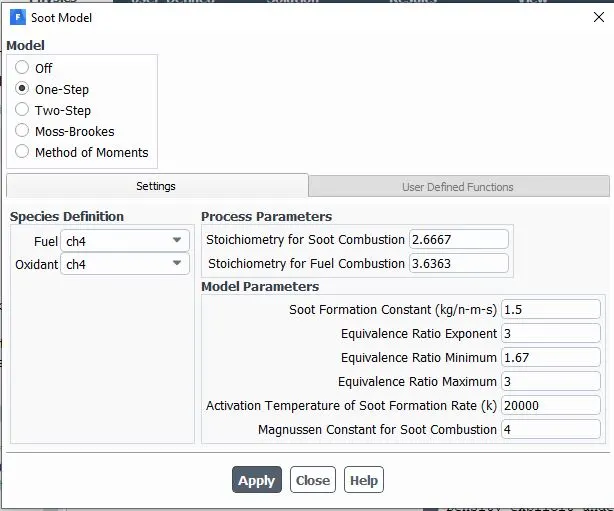
A One-Step Soot Model is used.

Boundary conditions:

• For Part-I, as there is no addition of Water h2O, the Air inlet will have a velocity of 0.5 m/s with a thermal temperature 300 k with species of 0.23 mass fraction of O2. For Fuel inlet, velocity is 80 m/s with thermal temperature 300 k and species of 1 mass fraction of ch4.

1. Air-inlet: Velocity = 0.5 m/s, T = 300 K, Mass fraction of O2 = 0.23

2. Fuel-inlet: Velocity = 80 m/s, T = 300 K, Mass fraction of CH4 = 1.

3. Outlet: Pressure Outlet, Guage pressure = 0.

4. Walls: Wall (No-slip wall)

• For Part-II, there is an addition of water in terms of 5, 15, 25, and 30% in fuel. so all the above conditions remains same with only change in fuel inlet species with 0.05 , 0.15 , 0.25 , 0.3 mass fraction of h2O with ch4 of mass fraction 0.95 , 0.85 , 0.75 , 0.7 respectively. Air inlet species remains the same with a 0.23 mass fraction of O2.

1. Air-inlet: Velocity = 0.5 m/s, T = 300 K, Mass fraction of O2 = 0.23

2. Fuel-inlet: Velocity = 80 m/s, T = 300 K,

• Mass fraction of CH4 = 0.95, 0.85, 0.75, 0.7 for 5, 15, 25, and 30% of Water in Fuel respectively.
• Mass fraction of H2O = 0.05, 0.15, 0.25, 0.3 for 5, 15, 25, and 30% of Water in Fuel respectively.

3. Outlet: Pressure Outlet, Guage pressure = 0.

4. Walls: Wall (No-slip wall)

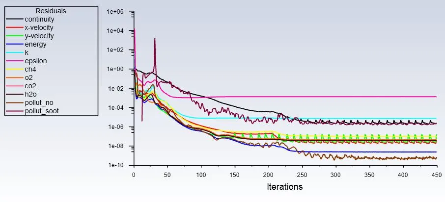
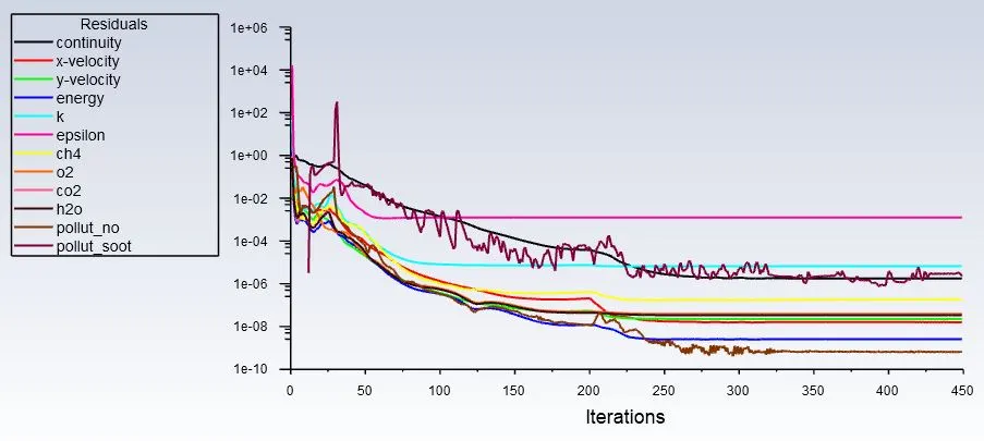
After applying all the settings explained above, the next step is to carry out Initialization and Run the simulation until the desired convergence achieved for all the required cases.

RESULTS AND DISCUSSION:

After completing all the procedures for the modeling and setup, this section provides the results of the simulation carried out with different physical inputs in 2 parts.

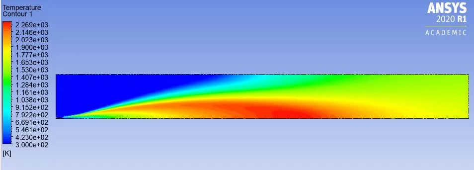
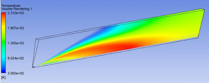
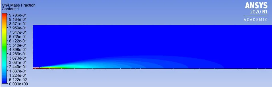
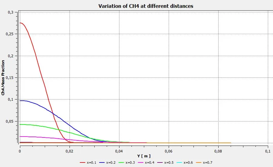
Part-I : CH4 = 1, O2 = 0.23

Residuals:

Temperature Contour with Volume Rendering:

Mass fraction of CH4 along with chart at varying distances:

Mass fraction of CO2 along with chart at varying distances:

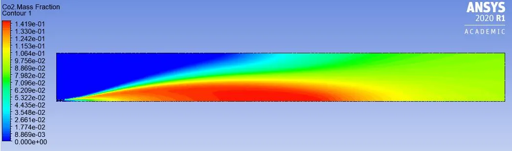
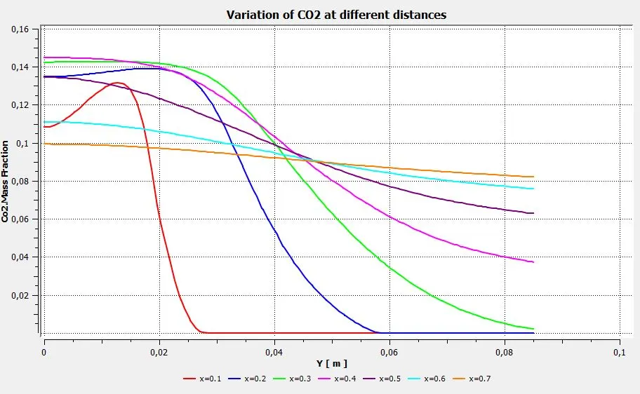
Mass fraction of O2 along with chart at varying distances:

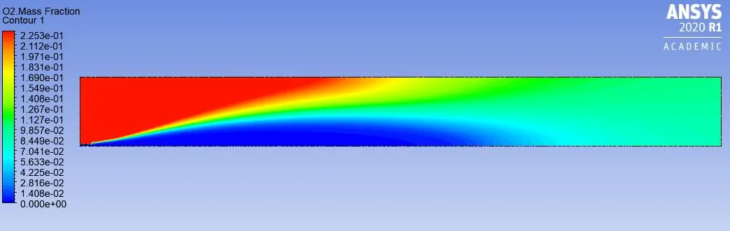
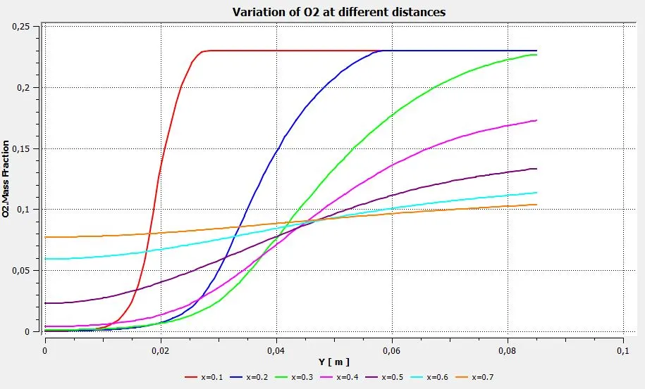
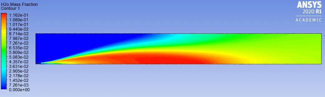
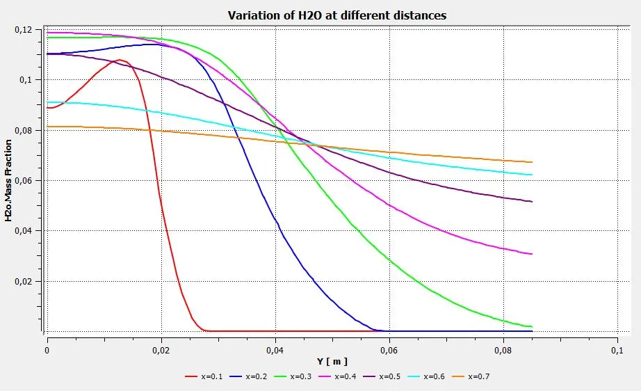
Mass fraction of H2O along with chart at varying distances:

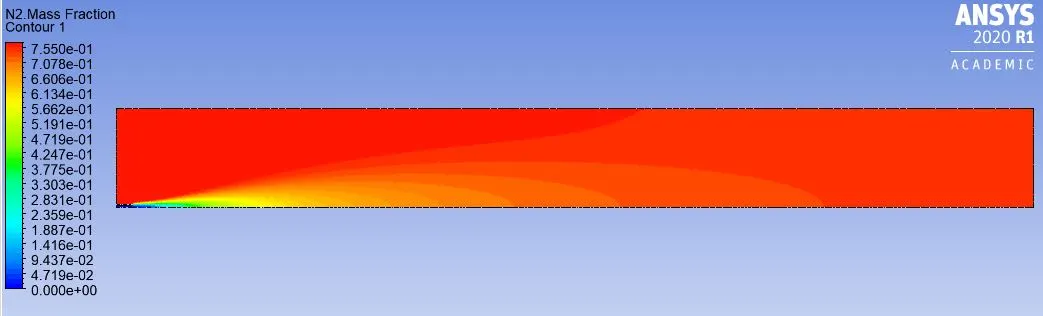
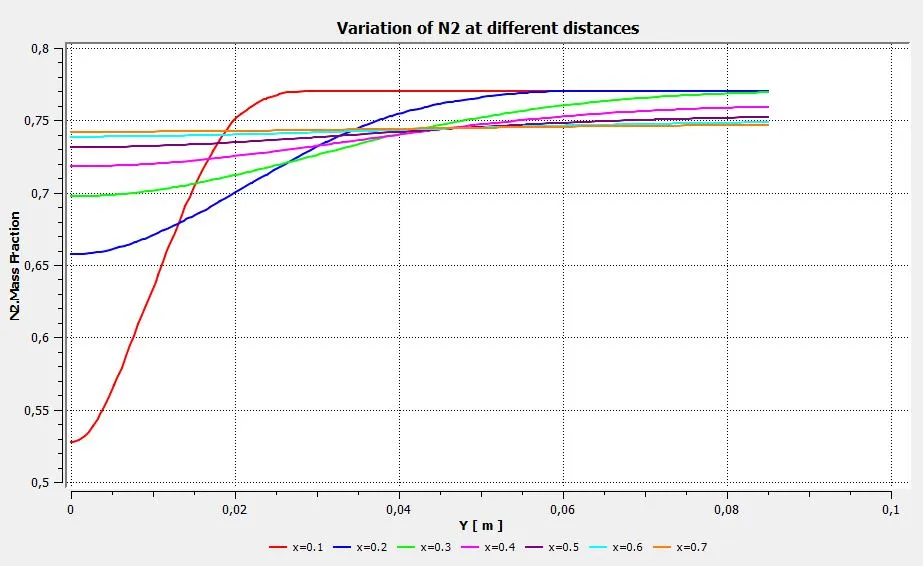
Mass fraction of N2 along with chart at varying distances:

Mass fraction of NOx along with chart at varying distances:

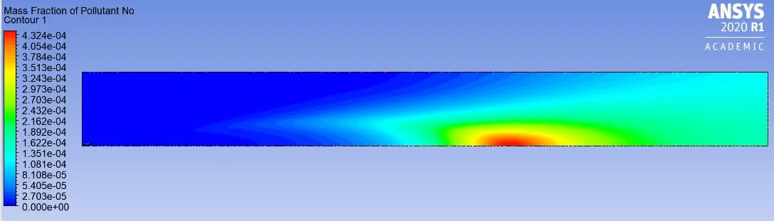
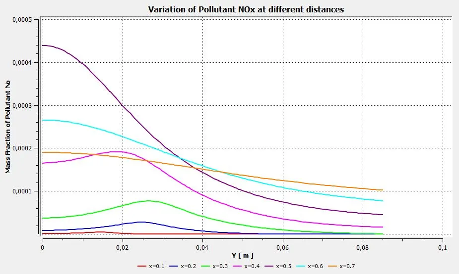
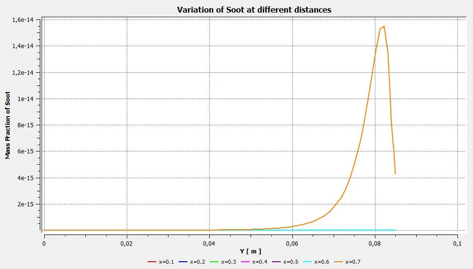
Mass fraction of Soot along with chart at varying distances:

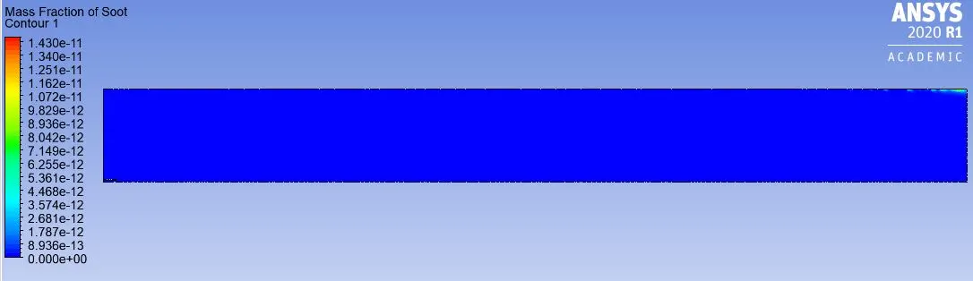
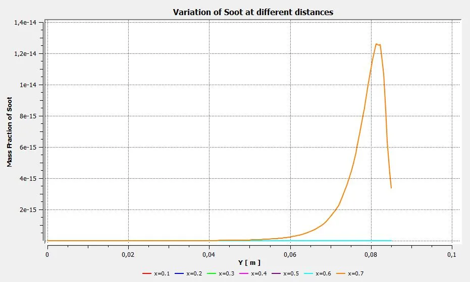
Part-II :

Case 1: CH4=0.95, H2O = 0.05, O2 = 0.23 (5% Water in Fuel).

Residuals:

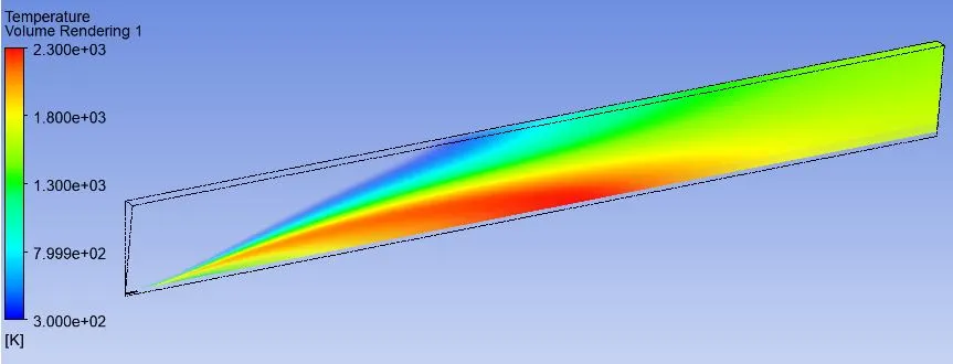
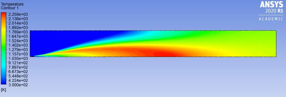
Temperature Contour with Volume Rendering:

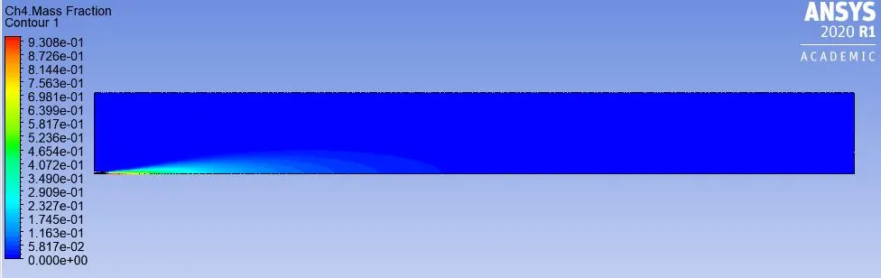
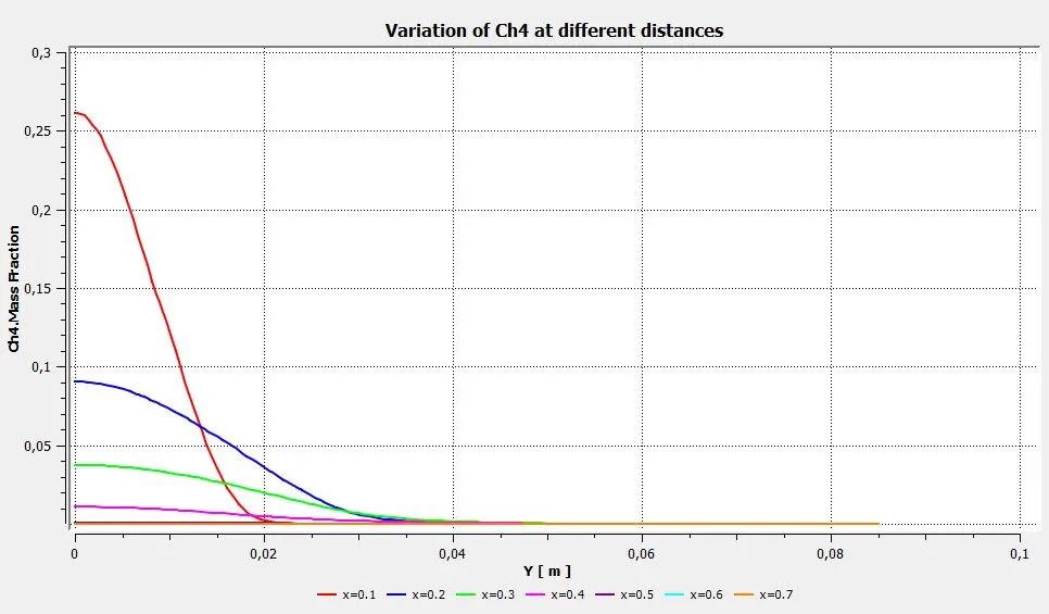
Mass fraction of CH4 along with chart at varying distances:

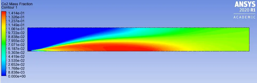
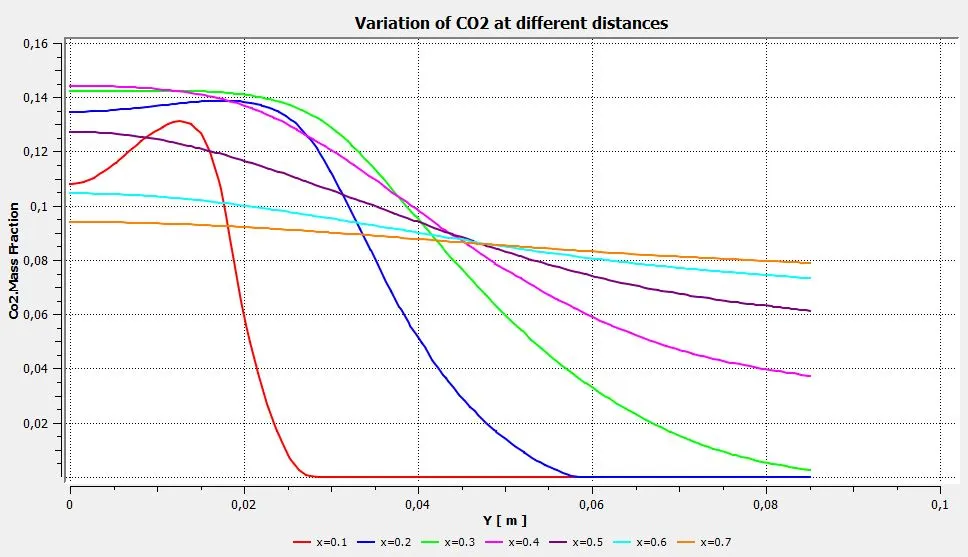
Mass fraction of CO2 along with chart at varying distances:

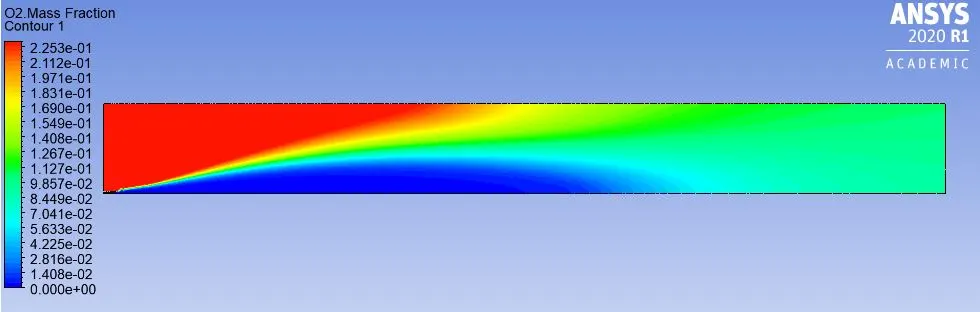
Mass fraction of O2 along with chart at varying distances:

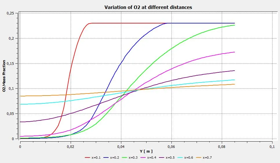
Mass fraction of H2O along with chart at varying distances:

Mass fraction of N2 along with chart at varying distances:

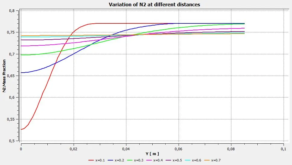
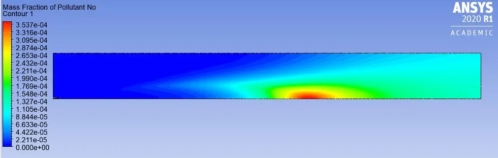
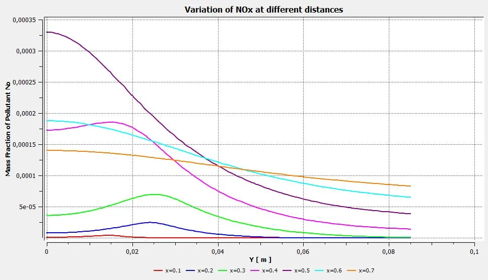
Mass fraction of NOx along with chart at varying distances:

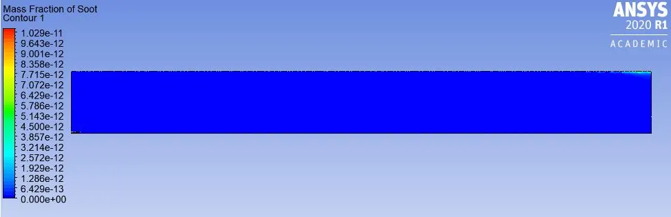
Mass fraction of Soot along with chart at varying distances:

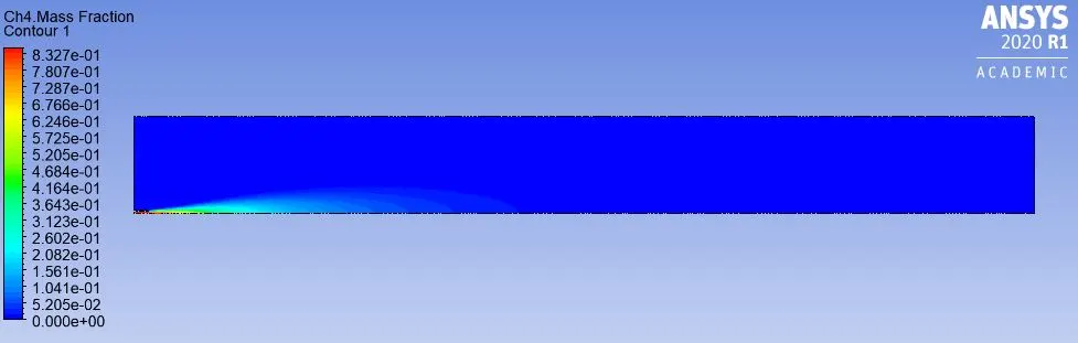
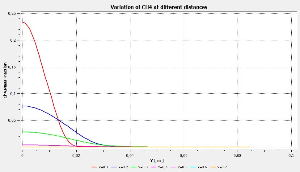
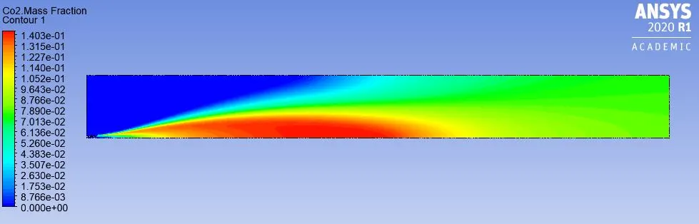
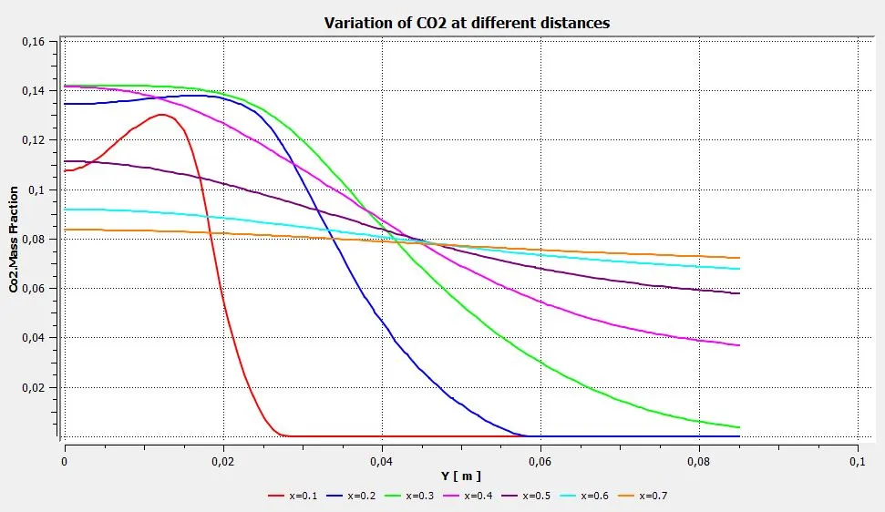
Case 2: CH4=0.85, H2O = 0.15, O2 = 0.23 (15% Water in Fuel).

Residuals:

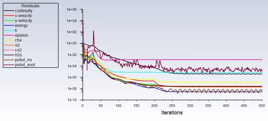
Temperature Contour with Volume Rendering:

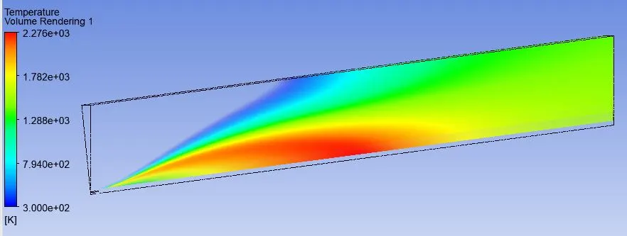
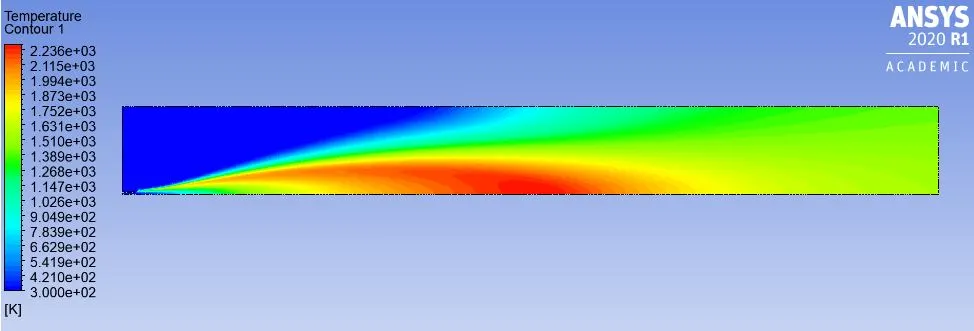
Mass fraction of CH4 along with chart at varying distances:

Mass fraction of CO2 along with chart at varying distances:

Mass fraction of O2 along with chart at varying distances:

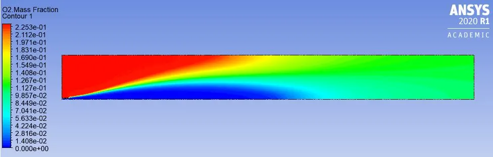
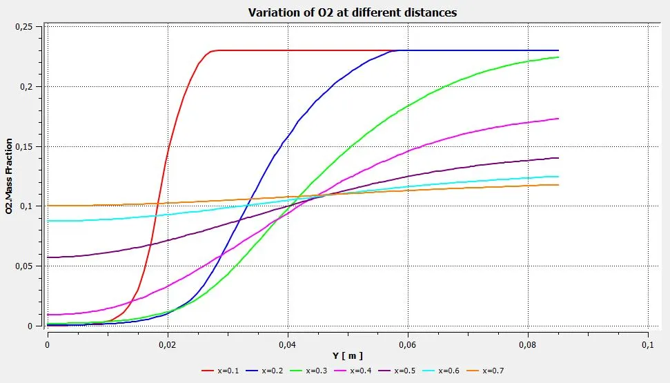
Mass fraction of H2O along with chart at varying distances:

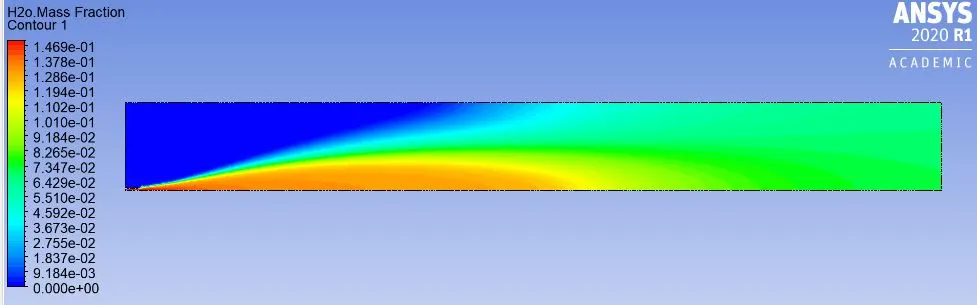
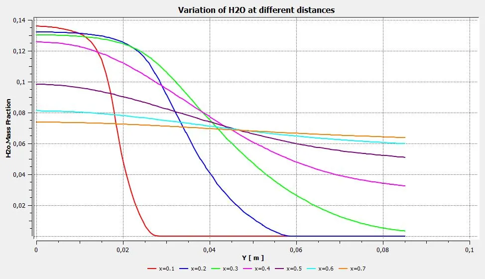
Mass fraction of N2 along with chart at varying distances:

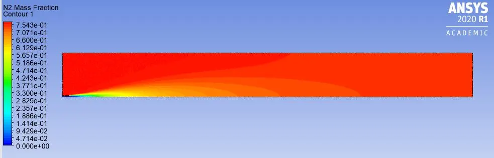
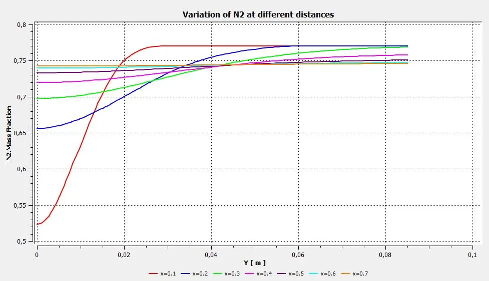
Mass fraction of NOx along with chart at varying distances:

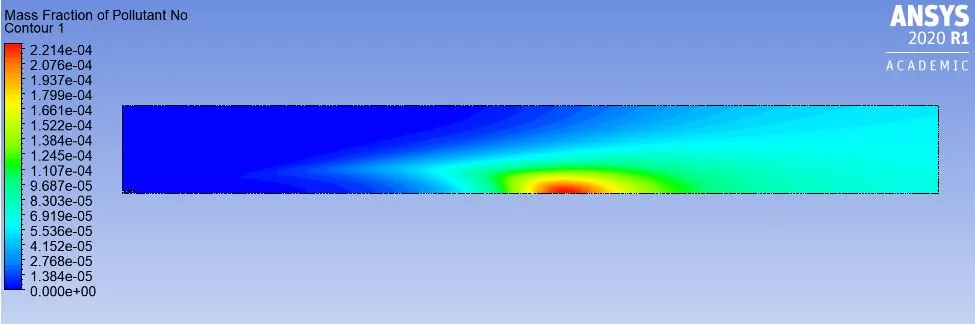
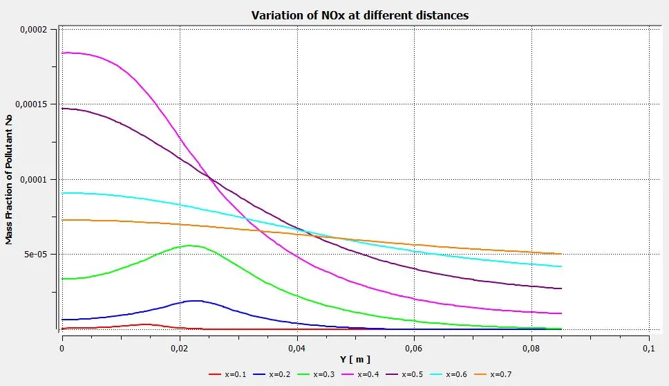
Mass fraction of Soot along with chart at varying distances:

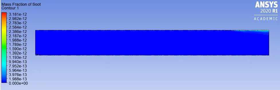
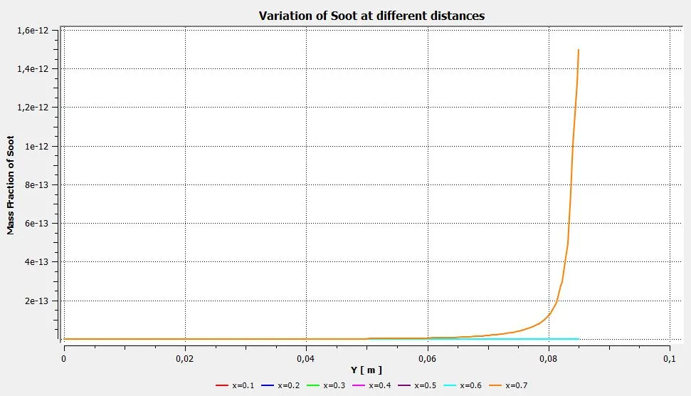
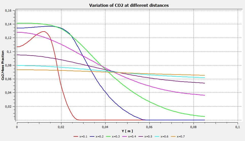
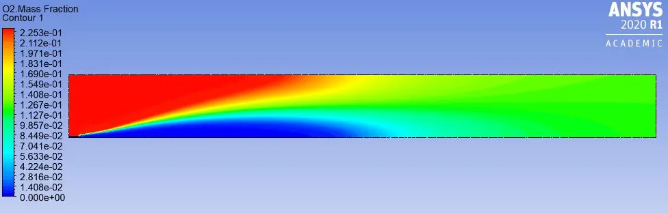
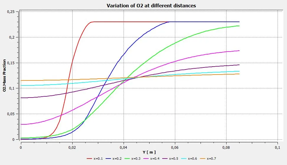
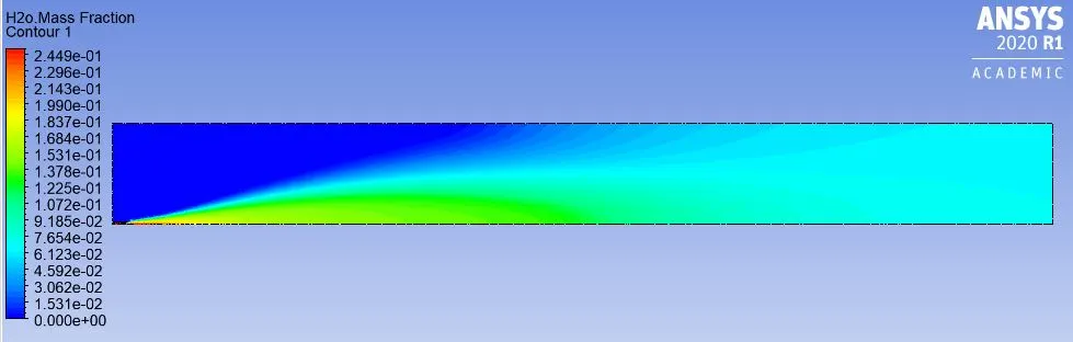
Case 3: CH4=0.75, H2O = 0.25, O2 = 0.23 (25% Water in Fuel).

Residuals:

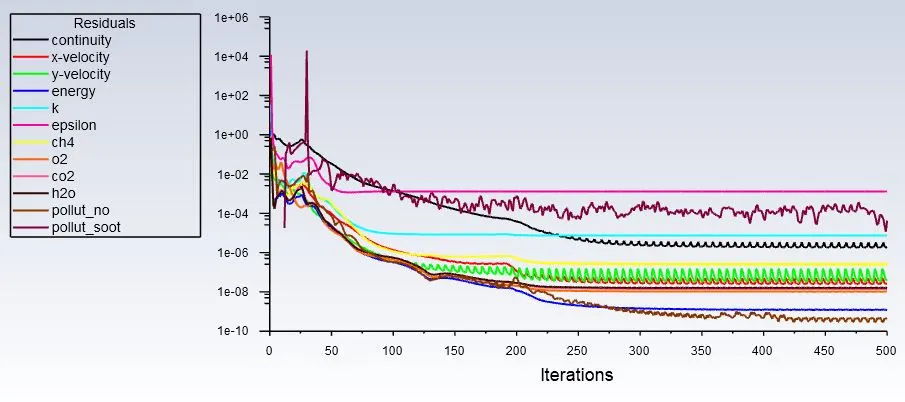
Temperature Contour with Volume Rendering:

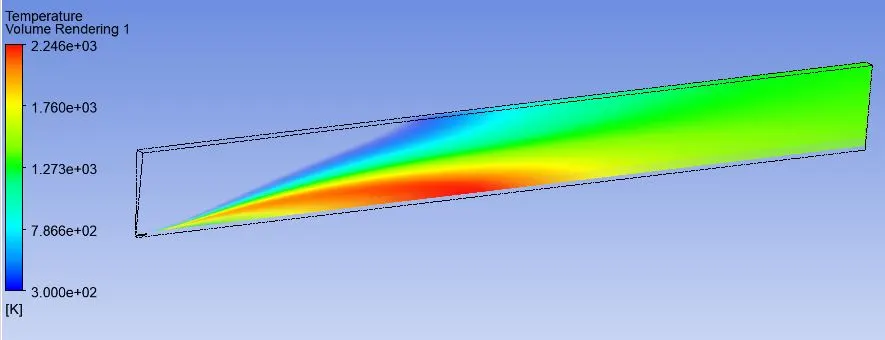
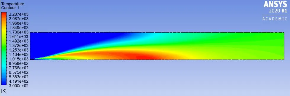
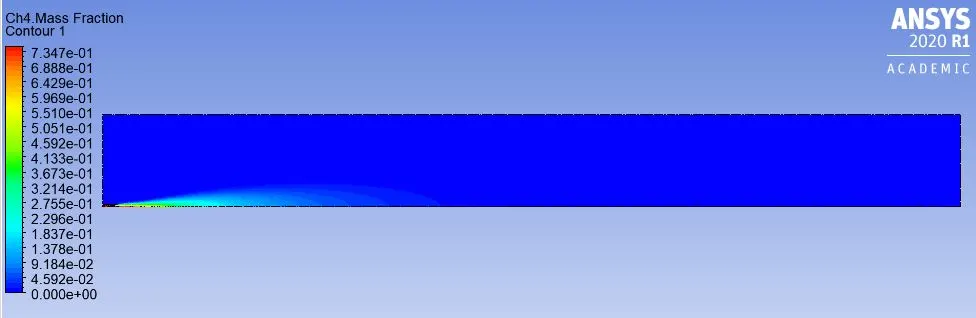
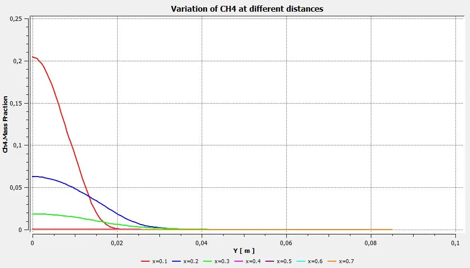
Mass fraction of CH4 along with chart at varying distances:

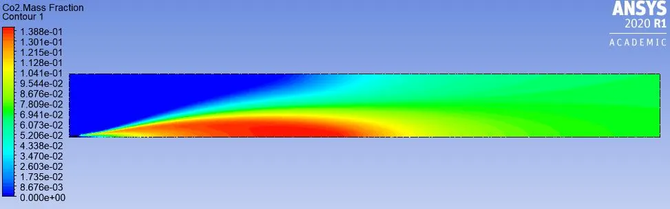
Mass fraction of CO2 along with chart at varying distances:

Mass fraction of O2 along with chart at varying distances:

Mass fraction of H2O along with chart at varying distances:

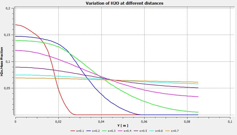
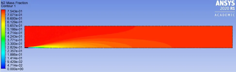
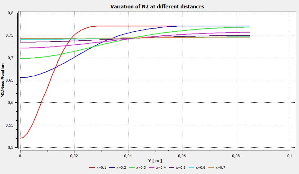
Mass fraction of N2 along with chart at varying distances:

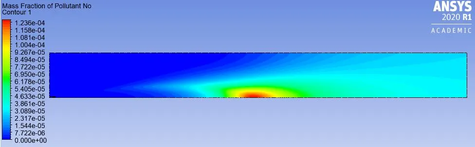
Mass fraction of NOx along with chart at varying distances:

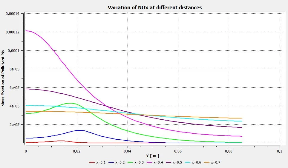
Mass fraction of Soot along with chart at varying distances:

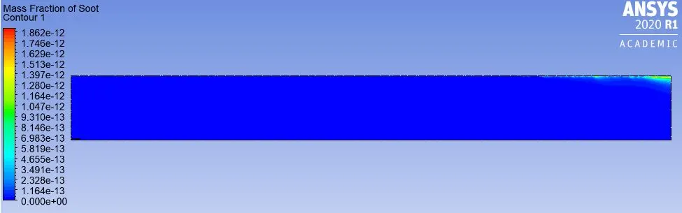
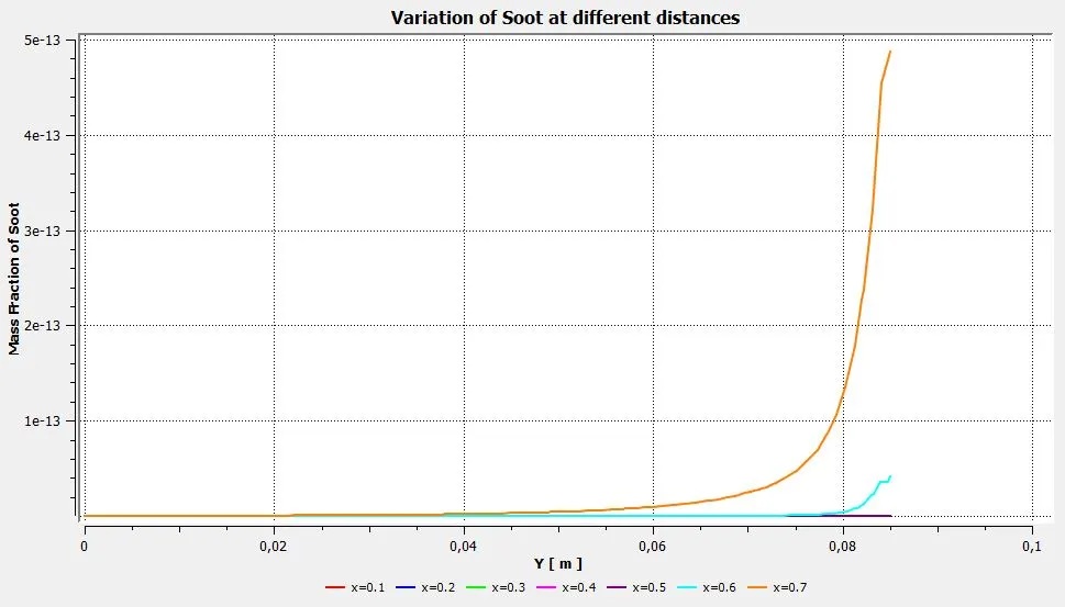
Case 4: CH4=0.7, H2O = 0.3, O2 = 0.23 (30% Water in Fuel).

Residuals:

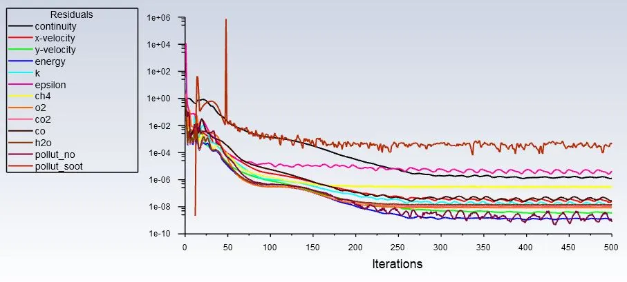
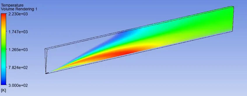
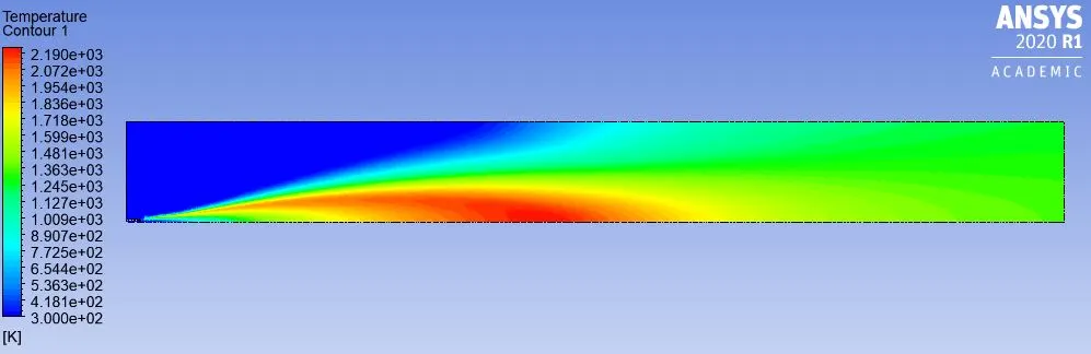
Temperature Contour with Volume Rendering:

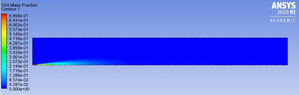
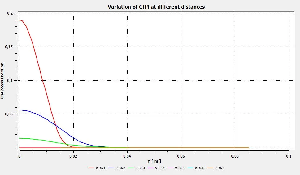
Mass fraction of CH4 along with chart at varying distances:

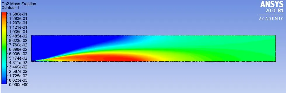
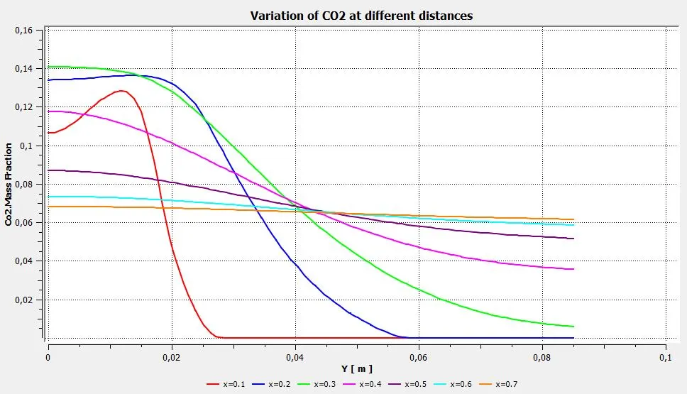
Mass fraction of CO2 along with chart at varying distances:

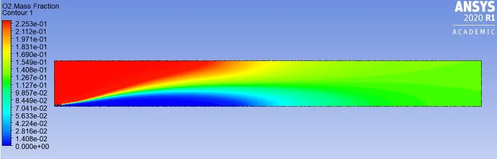
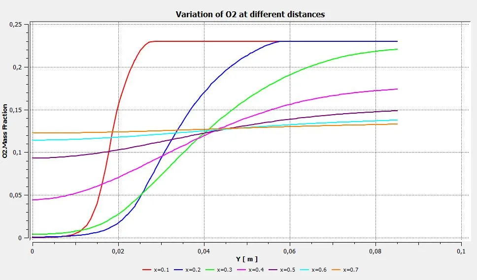
Mass fraction of O2 along with chart at varying distances:

Mass fraction of H2O along with chart at varying distances:

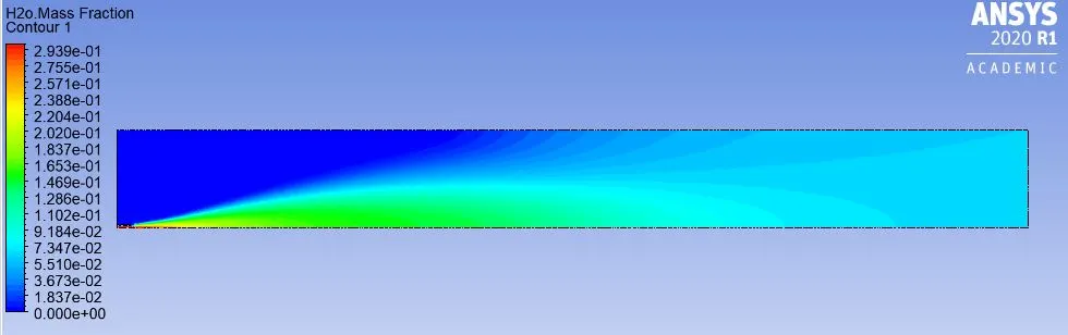
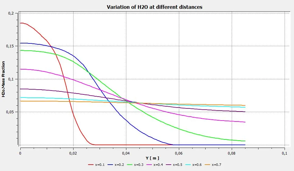
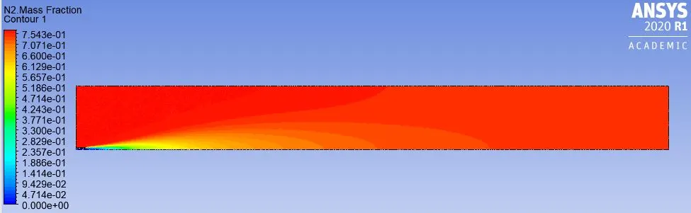
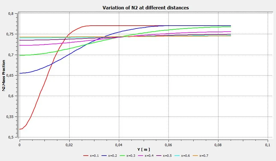
Mass fraction of N2 along with chart at varying distances:

Mass fraction of NOx along with chart at varying distances:

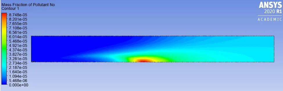
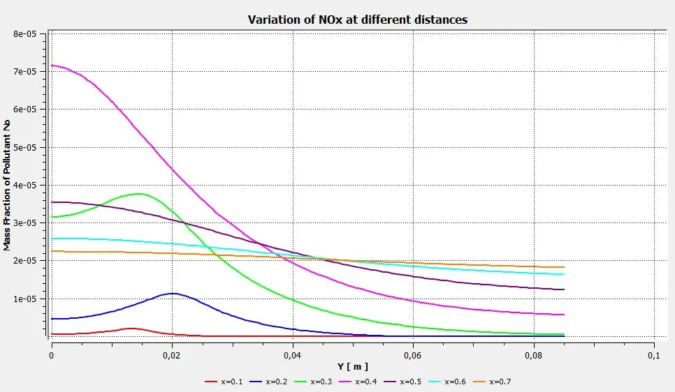
Mass fraction of Soot along with chart at varying distances:

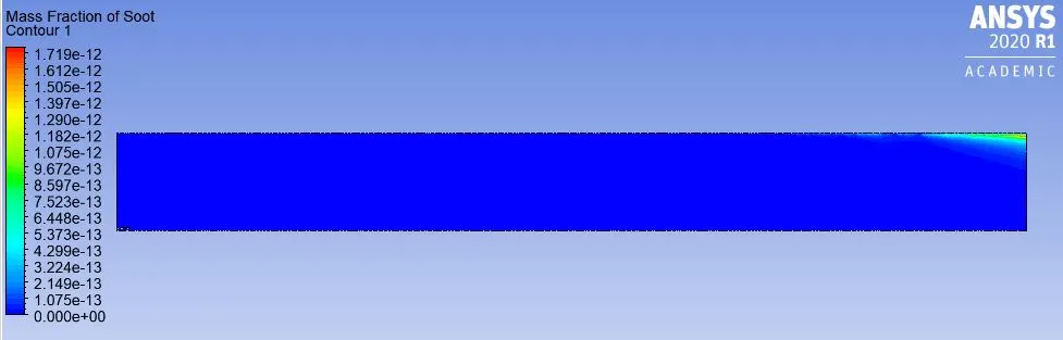
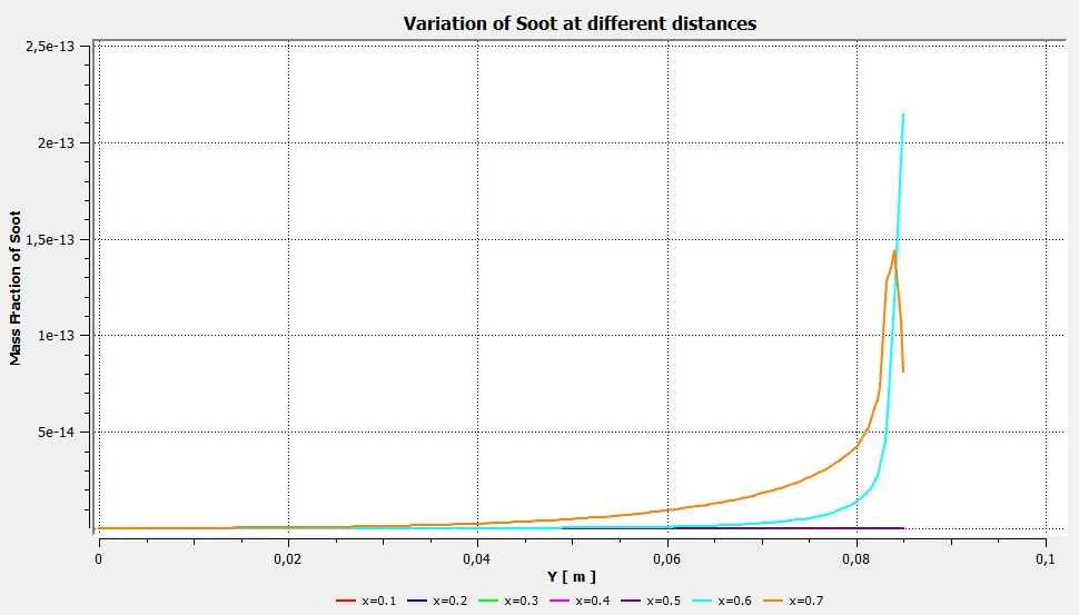
Comparison of Results for NOx and Soot Mass fraction at Outlet for all Cases:

Addition of Water in Fuel	Mass fraction of NOx at Outlet	Mass fraction of Soot at Outlet
No	4.324e-04	1.430e-11
5%	3.537e-04	1.029e-11
15%	2.214e-04	3.181e-12
25%	1.236e-04	1.862e-12
30%	8.748e-05	1.719e-12

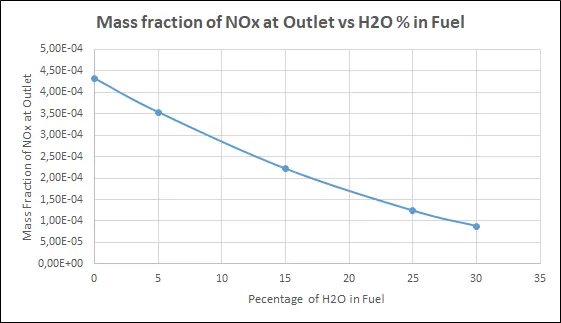
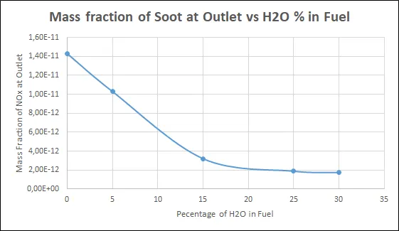
Plots of Comparison of Mass fraction for NOx and Soot with the addition of Water in a Fuel:

Conclusion:

After running the simulation for both the parts, there are few conclusions that can be drawn out. The parts consist of different setup with the first being without the addition of H2O in Fuel and the second being with the different proportion of water in fuel from 5% to 30%.

1) As can be observed from the first part of a simulation, the pollutant NOx and soot are getting formed at the outlet of the combustor as can be seen in the graphs and table above. Such formation has harmful effects on the environment and humans. The stringent government norms also demand the least formation of Nox and soot and to satisfy those requirements, it needs to check the effect of adding the water in the fuel.

2) From table and graphical representations, we can see that in the second part, the value of the mass fraction of NOx decreases with an increase in addition to water (H2O) in Fuel, which is great according to government norms with a reduction of NOx formation.

3) We can also observe that the mass fraction of soot reduces with an increase in the addition of water. Thus we can conclude that Combustion simulation is performed successfully.