CURVE FITTING USING MATLAB
AIM:
1.To Write code to fit a linear and cubic polynomial for the Cp data.
2.Plot the linear and cubic fit curves along with the raw data points.
3.To Write a code to show splitwise method.
4.To Explain the parameters used to measure the fitness characteristics for both the curves.
OBJECTIVE:
1.To Write code to fit a linear and cubic polynomial for the Cp data.
2.Plot the linear and cubic fit curves along with the raw data points.
3.To Write a code to show splitwise method which improves the accuracy .
4.To find whether the curve is good fit or not.
Theory:
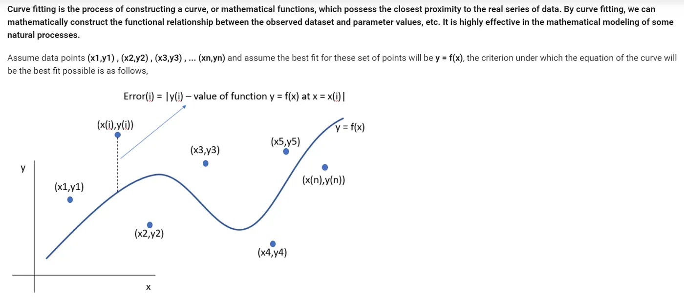
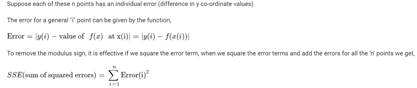
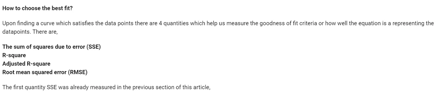


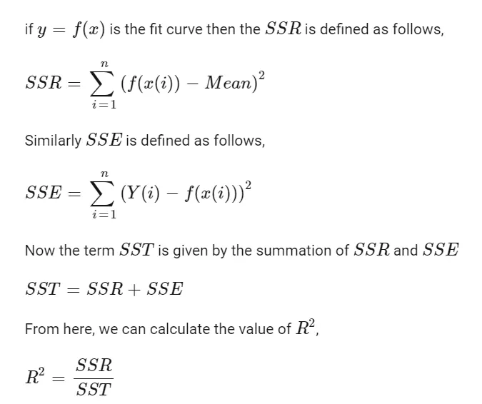
PROCEDURE:
- For solving objective 1 & 2 in matlab:
1. Intially we need to write a code to solve the linear and cubic polynomials using the data taken from the dataset using loaddata matlab command.
2.After this we need to use inbuilt matlab commands namely POLYFIT & POLYVAL in order to solve the linear & cubic equation by taking order 1 &3 respectively.
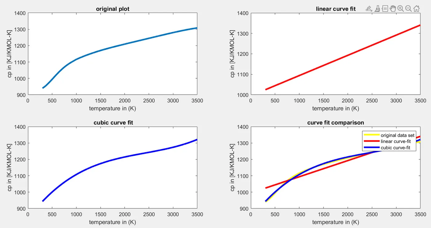
3.After solving the equation we need to plot the data namely (cp and temperature ) and also the predicted values of cp1 & cp2.
4. Then we keep legends and also xlabel and ylabel to make the plot detailed.
The matlab code for this is shown below:
clear all;
close all;
clc;
%% Extracting the data
cp_data = load('data');
temperature = cp_data(:,1);
cp = cp_data(:,2);
subplot(2,2,1);
plot(temperature,cp,'linewidth',3);
xlabel('temperature in (K)');
ylabel('cp in [KJ/KMOL-K]');
title('original plot');
%% curve fitting for linear polynomial
%% y = mx+c
coeff = polyfit(temperature,cp,1);
predicted_cp1 = polyval(coeff,temperature);
subplot(2,2,2);
plot(temperature,predicted_cp1,'linewidth',3,'color','r');
xlabel('temperature in (K)');
ylabel('cp in [KJ/KMOL-K]');
title('linear curve fit');
%% curve fitting for cubic polynomial
%% y = Ax^3+Bx^2+cX+D
coeff = polyfit(temperature,cp,3);
predicted_cp2 = polyval(coeff,temperature);
subplot(2,2,3);
plot(temperature,predicted_cp2,'linewidth',3,'color','b');
xlabel('temperature in (K)');
ylabel('cp in [KJ/KMOL-K]');

%% plotting the curves together
title(' cubic curve fit');
subplot(2,2,4)
plot(temperature,cp,'linewidth',3,'color','y');
hold on;
%%subplot(2,1,2);
plot(temperature,predicted_cp1,'linewidth',3,'color','r');
hold on;
plot(temperature,predicted_cp2,'linewidth',3,'color','b');
hold off;
title('curve fit comparison');
xlabel('temperature in (K)');
ylabel('cp in [KJ/KMOL-K]');
legend('original data set','linear curve-fit','cubic curve-fit');
Plots for the obective 1 &2 :
ERROR REPORT :
During this i have encountered a problem and i have attached the screen shot below:
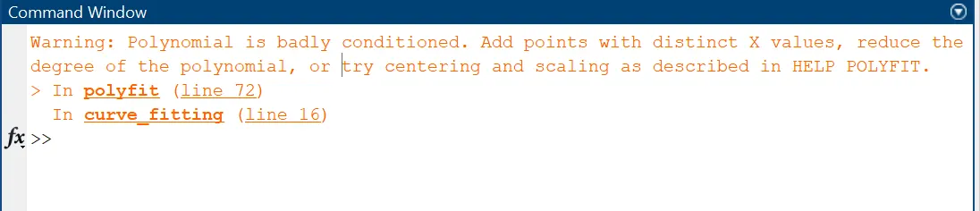
Rectified this error by using the split wise method approach and also by reducing the degree of the polynomial to 2.
Procedure for solving the split wise method is as follows:
1. Initially using clear all , close all & clc we have cleared the entire data.
2. We have taken the data from the data file and assigned them to the temperature and cp .
3. For temperature instead of solving all at a time we have used Split -Wise method to solve the
equation.
4.Temperature & cp is an array of 3200*1 so we solved it by splitting it into 4 intervals namely
(1,800),(801,1600),(1601,2400),(2401,3200)
5.Now using this we have used polyfit and polyval command at each interval and solved it and also plotted the curve accordingly.
6. Then we keep legends and also xlabel and ylabel to make the plot detailed.
The matlab code for this is shown as follows:
clear all;
close all;
clc;
%% Extracting the data
cp_data = load('data');
temperature = cp_data(:,1);
cp = cp_data(:,2);
subplot(2,2,1);
plot(temperature,cp,'linewidth',3);
xlabel('temperature in (K)');
ylabel('cp in [KJ/KMOL-K]');
title('original plot');
%% curve fitting for linear polynomial
%% y = mx+c
coeff = polyfit(temperature,cp,1);
predicted_cp1 = polyval(coeff,temperature);
subplot(2,2,2);
plot(temperature,predicted_cp1,'linewidth',3,'color','r');
xlabel('temperature in (K)');
ylabel('cp in [KJ/KMOL-K]');
title('linear curve fit');
%% curve fitting for cubic polynomial and splitting the temperature.
%% y = Ax^2+Bx+c
cp_data = load('data');
%% split 1
temperature1 = cp_data(1:800,1);
cp_1 = cp_data(1:800,2);
%% split 2
temperature2 = cp_data(801:1600,1);
cp_2 = cp_data(801:1600,2);
%% split 3
temperature3 = cp_data(1601:2400,1);
cp_3 = cp_data(1601:2400,2);
%% split 4
temperature4 = cp_data(2401:3200,1);
cp_4 = cp_data(2401:3200,2);
coeff1 = polyfit(temperature1,cp_1,2);
coeff2 = polyfit(temperature2,cp_2,2);
coeff3 = polyfit(temperature3,cp_3,2);
coeff4 = polyfit(temperature4,cp_4,2);
predicted_cp2_1 = polyval(coeff1,temperature1);
predicted_cp2_2 = polyval(coeff2,temperature2);
predicted_cp2_3 = polyval(coeff3,temperature3);
predicted_cp2_4 = polyval(coeff4,temperature4);
subplot(2,2,3);
plot(temperature1,predicted_cp2_1,'linewidth',3,'color','b');
hold on;
plot(temperature2,predicted_cp2_2,'linewidth',3,'color','b');
hold on;
plot(temperature3,predicted_cp2_3,'linewidth',3,'color','b');
hold on;
plot(temperature4,predicted_cp2_4,'linewidth',3,'color','b');
xlabel('temperature in (K)');
ylabel('cp in [KJ/KMOL-K]');
hold off;
%% plotting the curves together
title(' cubic curve fit');
subplot(2,2,4)
plot(temperature,cp,'linewidth',3,'color','r');
hold on;
%%subplot(2,1,2);
plot(temperature,predicted_cp1,'linewidth',3,'color','y');
hold on;
plot(temperature1,predicted_cp2_1,'linewidth',3,'color','b');
hold on;
plot(temperature2,predicted_cp2_2,'linewidth',3,'color','b');
hold on;
plot(temperature3,predicted_cp2_3,'linewidth',3,'color','b');
hold on;
plot(temperature4,predicted_cp2_4,'linewidth',3,'color','b');
hold off;
title('curve fit comparison');
xlabel('temperature in (K)');
ylabel('cp in [KJ/KMOL-K]');
legend('original data set','linear curve-fit','cubic curve-fit','location','southeast');
Plots for the obective 3 is shown below:
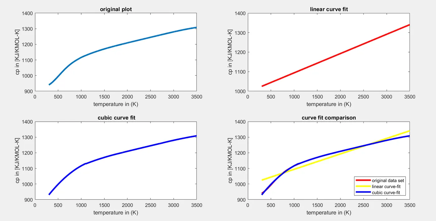
To solve objective 4 that is to find whether the given curve is good fit or not we used a matlab code to solve this
Procedure for solving the characteristics of the curve is as follows:
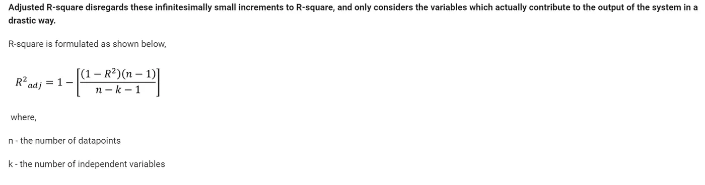
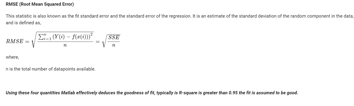
1. Using the formulaes available we have solved the SSE,SST,R^2,ADJUSTED R^2,RMSE for each and every interval .
2. After solving it using this values if R^2 value is greater than 0.95 the curve is known as good fit.
We can find this using 2 ways namely:
1.Through analytical way
2.Through CURVE FITTING TOOL
The matlab code using analytical way:
%% calculation for finding whether the choosen curve is good curve fit or not
%% for data set 1
%% finding sse
error1 = predicted_cp2_1-cp_1;

for i = 1:length(cp_1)
    sse1 = error1(i)^2;
    SSE1 = 0+error1(i)^2 ;
    sumcp_1 =cp_1(i);
end

%% to find mean for data set 1
n1 = length(cp_1);
mean1 = sumcp_1/n1;

%% ssr for data set 1
for k = 1:length(cp_1)
    ssr_1 = (predicted_cp2_1(i)-mean1)^2;
    SSR1 = 0+ssr_1;
end

%% finding SST
SST1 = SSR1 +SSE1;

%% calculating R^2
R_sq1 = SSR1/SST1 ;

%% adjusted r^2
%% no. of independent variables
j =1;
R_adj_sq1 = 1-(((1-R_sq1^2)*(n1-1))/(n1-j-1));

%% RMSE
RMSE1 = (SSE1/n1)^(0.5);


%% for data set 2
%% finding sse
error2 = predicted_cp2_2-cp_2;

for i = 1:length(cp_2)
    sse2 = error2(i)^2;
    SSE2 = 0+error2(i)^2 ;
    sumcp_2 =cp_2(i);
end

%% to find mean for data set 1
n2 = length(cp_2);
mean2 = sumcp_2/n2;

%% ssr for data set 2
for k = 1:length(cp_2)
    ssr_2 = (predicted_cp2_2(i)-mean2)^2;
    SSR2 = 0+ssr_2;
end

%% finding SST
SST2 = SSR2 +SSE2;

%% calculating R^2
R_sq2 = SSR2/SST2 ;

%% adjusted r^2
%% no. of independent variables
j =1;
R_adj_sq2 = 1-(((1-R_sq2^2)*(n2-1))/(n2-j-1));

%% RMSE
RMSE2 = (SSE2/n2)^(0.5);

%% for data set 3
%% finding sse
error3 = predicted_cp2_3-cp_3;

for i = 1:length(cp_3)
    sse3 = error3(i)^2;
    SSE3 = 0+error3(i)^2 ;
    sumcp_3 =cp_3(i);
end

%% to find mean for data set 3
n3 = length(cp_3);
mean3 = sumcp_3/n3;

%% ssr for data set 1
for k = 1:length(cp_3)
    ssr_3 = (predicted_cp2_3(i)-mean3)^2;
    SSR3 = 0+ssr_3;
end

%% finding SST
SST3 = SSR3 +SSE3;

%% calculating R^2
R_sq3 = SSR3/SST3 ;

%% adjusted r^2
%% no. of independent variables
j =1;
R_adj_sq3 = 1-(((1-R_sq2^3)*(n3-1))/(n3-j-1));

%% RMSE
RMSE3 = (SSE3/n3)^(0.5);


%% for data set 4
%% finding sse
error4 = predicted_cp2_4-cp_4;

for i = 1:length(cp_4)
    sse4 = error4(i)^2;
    SSE4 = 0+error4(i)^2 ;
    sumcp_4 =cp_4(i);
end

%% to find mean for data set 3
n4 = length(cp_4);
mean4 = sumcp_4/n4;

%% ssr for data set 4
for k = 1:length(cp_4)
    ssr_4 = (predicted_cp2_4(i)-mean4)^2;
    SSR4 = 0+ssr_4;
end

%% finding SST
SST4 = SSR4 +SSE4;

%% calculating R^2
R_sq4 = SSR4/SST4 ;

%% adjusted r^2
%% no. of independent variables
j =1;
R_adj_sq4 = 1-(((1-R_sq2^4)*(n4-1))/(n4-j-1));

%% RMSE
RMSE4 = (SSE3/n4)^(0.5);

%% loop for determining whether the given fit is good fit or not using R^2

if [R_sq1 > 0.95 ,R_sq2 > 0.95,R_sq3 > 0.95 ,R_sq4 > 0.95]
    disp('GIVEN FIT IS A GOOD FIT ');
else
    disp('GIVEN FIT IS NOT A GOOD FIT');
end
Using Curve fit Tool Box:
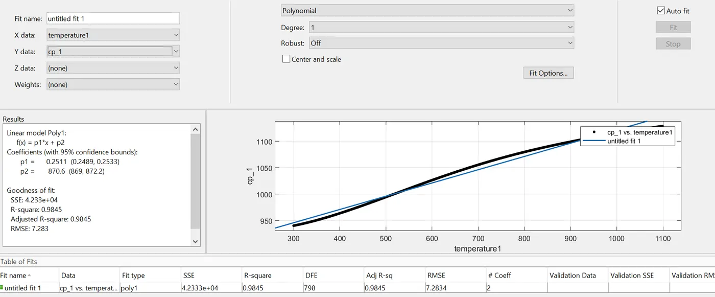
1) Linear Curve fit
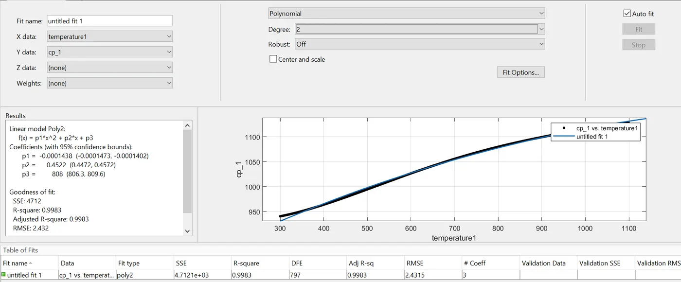
Quadratic curve fit:
- How to make a curve fit perfectly?
Answer:We can make a curve fit perfectly by reducing the error between the original values and the predicted values so that the curve fits perfectly.
2.How to get the best fit?
Answer:To get the best fit we use 4 methods as mentioned already above namely:
1.SSE
2.SST
3.R^2
4.ADJUSTEDR^2
5.RMSE
Using this techniques we can predict whether the fit is best fit or not
If R^2 value is greater than 0.95 than the fit is considered to be the best fit
3.What could be done to improve the cubic fit?
Answer:By doing split wise method and also by using techniques like scaling and centering we can improve the cubic fit and also by splitting array into parts and solving them can also improve the cubic fit.
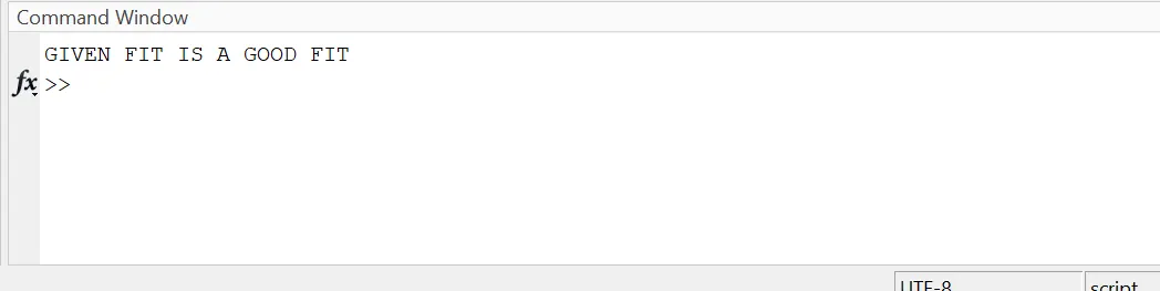
OUTPUT:
CONCLUSION:
Using the given data of CP and Temperature we have solved the linear and cubic fit for them and made it more accurate by using split wise method and also found the characteristics of the curve whether it is good fit or not using analytical and curve fit tool box.
The end result for the fit is Good as the value of R^2 is 0.99 which is greater than 0.95.
REFERENCES:
https://projects.skill-lync.com/projects/Curve-Fitting-and-criterion-to-choose-best-fit-41860