Week 3 - Solving second order ODEs

AIM: To write a matlab code that can solve second order ODE with an example of simple pendulum.

OBJECTIVE:

1. To write a Matlab code that can solve second order ODE using inbuilt matlab solver ODE45 and plot the end results of angular displacement and angular velocity with respect to time.

2. After successfully completing 1st objective we need to simulate the animation by taking values of theta and plotting them.

3. After successfully plotting the end results, we need to create a video file, '.AVI' and need to complete the simulation.

FORMULA:

Using the trigonometric relations of simple pendulum we need to find end points of pendulum rod.

(x0,y0)=(0,0)

(x1,y1)=(x0+lsintheta,y0-lcostheta)

PROCEDURE:

1. Intially we need to solve second order ODE by converting into two first order ODE's namely:

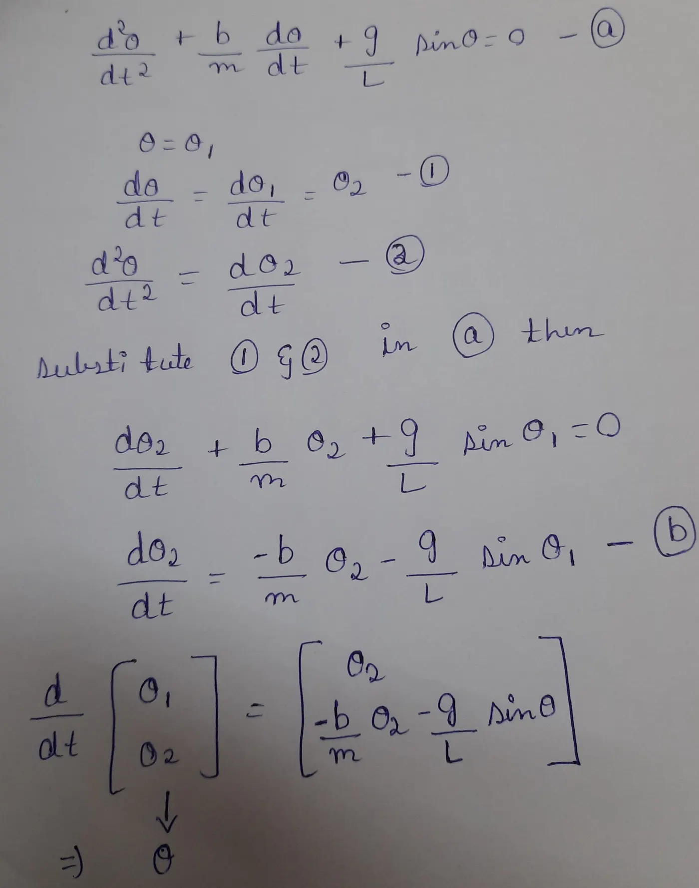
2. Using the below function and matlab code we solve and plot the end results of angular displacement and angular velocity with respect to time.

3. Initial conditions such a length,mass of the ball,gravity,damping coefficient are given and using above formulae we find the both end points of pendulum rod.

The matlab code for this is shown below:

clear all;
close all;
clc;
%% Inputs of the pendulum
l=1;
m=1;
b=0.05;
g=9.81;
cnt  =1;
%% initial conditions(Angular-displacement,Angular-Velocity)
theta_0 = [0;3];

%% time plots
t_span = linspace(0,20,50);

%% solving ODE(ODE45 Command)
[t,theta] = ode45(@(t,theta) ode_funct(t,theta,l,m,b,g),t_span,theta_0);

%% plotting  the curve
figure(1);
plot(t,theta(:,1))
grid on;
hold on;
plot(t,theta(:,2))
xlabel('time');
ylabel('plot');
legend('Angular displacement','Angular Velocity');

%% for making an animation
DISP_THETA = theta(:,1); 
for j = 1:length(DISP_THETA)
     theta2 =DISP_THETA(j);
   %% time = TIME(j);  
x0=0;
y0=0;
x1=x0+l*sind(theta2);
y1=y0-l*cosd(theta2); 
figure(2);
plot([-1,1],[0,0],'linewidth',4,'color','y');
hold on;
plot([x0 x1],[y0 y1],[x1,x1],[y1,y1],'o','markersize',10,'markerfacecolor','r','linewidth',3,'color','b');
hold off;
xlabel('X-Axis');
ylabel('Y-Axis');
axis([-0.4 0.4 -1 1]);
pause(0.1);
M(cnt) = getframe(gcf);
cnt = cnt + 1; 
end

%% Animation of the plot 
movie(M);
v = VideoWriter('Motion of a Simple_Pendulum.avi');
open(v);
writeVideo(v,M);
close(v);

Function for the Matlab code is given below:

function [dtheta_dt] = ode_funct(t,theta,l,m,b,g)

theta1 = theta(1);
theta2 = theta(2);
dtheta1_dt = theta2;
dtheta2_dt = -(b/m)*theta2-(g/l)*sind(theta1);
[dtheta_dt] = [dtheta1_dt ; dtheta2_dt];
end

REPORT :

During this i have encountered many problems and i have attached some of the screen shots below:

1.During plotting i used multiple coordinates in a single plot command where i used linspace and color which in general is not possible.

2.During taking the end co-ordinates (x1,y1). I considered angle theta with x-axis which resulted in plot as shown below.

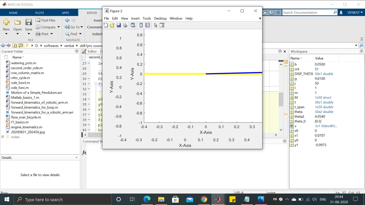
-Rectified this my changing the theta(angle) with respect to y axis and derived the coordinates

3.During variable declaration and usage matlab is case -sensitive but i havent followed this which ended up as error.

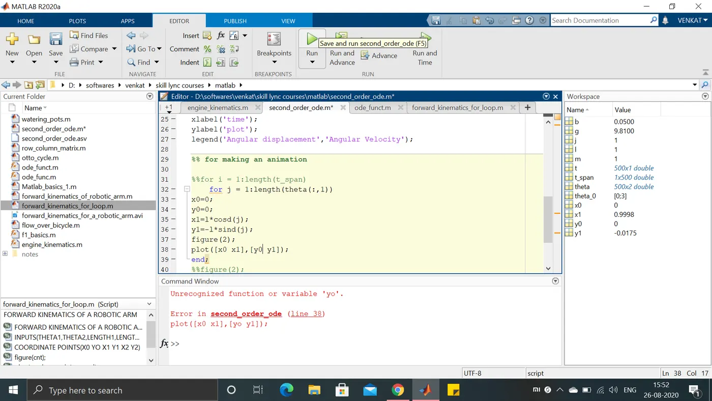
In this we have used inbuilt Matlab functions in order to generate a Video file of the output :

OUTPUT:

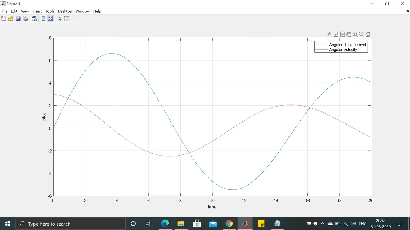
1. Plots for angular-velocity and angular-displacement where made with respect to that of the time and the plot is shown below:

2. The end result of simulation is given in the link below:

https://youtu.be/HXs2U2pR0rc

CONCLUSION:

1. We have succesfully solved second order ODE with using matlab solver using inbuilt matlab solver ODE45.
2. We have succesfully plotted the motion of pendulum.