Curve Fitting using MATLAB
Curve fitting
Curve fitting is the process of constructing a curve, or mathematical functions, which posses the closest proximity to the real dataset. Curve fitting can construct a mathematical relation between the observed dataset and parameter values. It is highly effective in the mathematical modeling of some natural processes.
Curve fitting can involve either interpolation, where an exact fit to the data is required, or smoothing, in which a "smooth" function is constructed that approximately fits the data. A related topic is regression analysis, which focuses more on questions of statistical inference such as how much uncertainty is present in a curve that is fit to data observed with random errors.
Regression analysis is primarily used for two conceptually distinct purposes. First, regression analysis is widely used for prediction and forecasting, where its use has substantial overlap with the field of machine learning. Second, in some situations, regression analysis can be used to infer causal relationships between the independent and dependent variables. Importantly, regressions by themselves only reveal relationships between a dependent variable and a collection of independent variables in a fixed dataset.
Finding the degree of polynomial function to fit the dataset
Polynomial regression is a form of regression analysis in which the relationship between the independent variable x and the dependent variable y is modelled as an nth degree polynomial in x. Polynomial regression fits a nonlinear relationship between the value of x and the corresponding conditional mean of y.
The first degree polynomial equation
`y=ax+b`
is a line with slope '`a`'. A line will connect any two points, so a first degree polynomial equation is an exact fit through any two points with distinct x coordinates.
If the order of the equation is increased to a second degree polynomial, the following results:
`y=ax^{2}+bx+c`
This will exactly fit a simple curve to three points.
If the order of the equation is increased to a third degree polynomial, the following is obtained:
`y=ax^{3}+bx^{2}+cx+d`
This will exactly fit four points.
A more general statement would be to say it will exactly fit four constraints. Each constraint can be a point, angle, or curvature (which is the reciprocal of the radius of an osculating circle). Angle and curvature constraints are most often added to the ends of a curve, and in such cases are called end conditions.
Solving polynomial function and finding the goodness of fit
How to choose the best fit
Upon finding a curve that satisfies the data points there are 4 methods to measure the goodness of fit criteria.
The 4 methods are:-
1. The Sum of Square due to Error (SSE)
2. R-Square
3. Adjusted R-Square
4. Root Mean Square Error
1. The Sum of Square due to Error (SSE)
Let the function of the form `y=f(x)`
Assume the data points (x1,y1),(x2,y2),.....(xn,yn) are plotted as the values of function `y=f(x)`
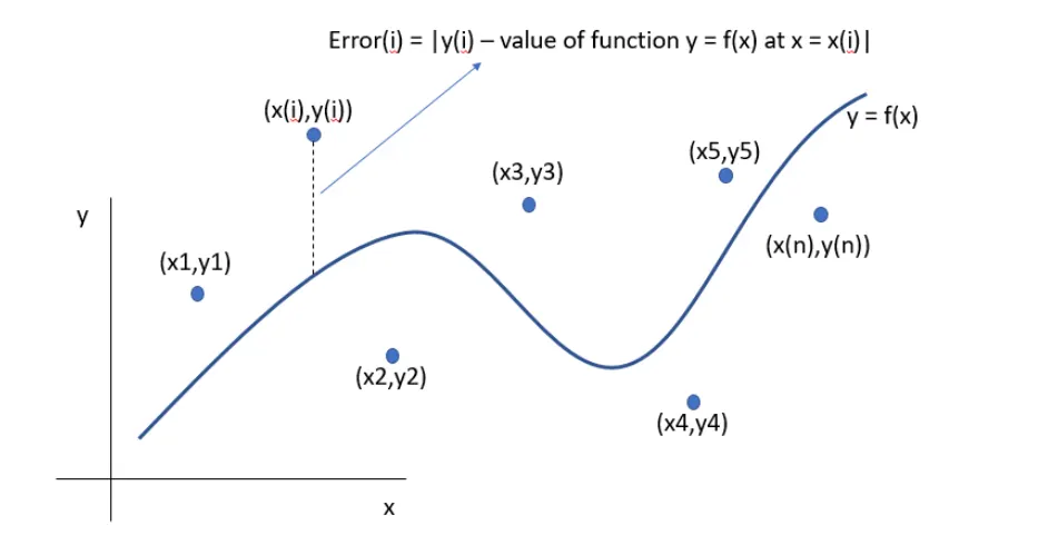
Suppose each of these points has an individual error (difference in y co-ordinate values) with the curve. The error at any general point 'i' can be given by the function,
`Er ro r(i)=|y_i-f(x_i)|`
where
`y_i` =value of y at i (corresponding value on curve at instant i)
`f(x_i)` = value of function `f(x)` at x=i
To remove the modulus sign, it is effective to take square of error.
The square of error of all the terms ranging from 1 to n is called Sum of Squared Error (`SSE`).
`SSE=sum_(i=1)^nEr ro r_i^2`
Assume the proposed equation is nth degree polynomial of the form,
`f(x)=A_1+A_2.x+A_3.x^2+...+A_n.x^(n-1)`
when we differentiate the (`SSE`) with each coefficient of the proposed equation `f(x)` respectively and equate to zero, we can find the minima and the value of coefficients of `f(x)`.
`Coefficient(f(x))[[(dS S E)/(dA_1)=0],[(d S S E)/(dA_1)=0],[.],[.],[.],[(dS S E)/(dA_n)=0]]`
2. R-Square
R-Square measures how successful the fit is in explaining the variation of the data. It is square of the correlation between the response value and the predicted response. It is also called the square of the multiple correlation coefficient and the coefficient of multiple determination.
It means that the higher the value of R-Square the better the fit, the lower it is the lousier the fit. The Value of R-Square ranges from 0 to 1.
0 for the worst possible fit and 1 for the best possible fit.
The value of R-Square can be calculated using the formula
``R^2=(SSR)/(SST)` where
SSR = is the sum of square of the difference between the values of the fitting function at a given point and the arithmetic mean of the data set.
SST= is the squared differences between the observed dependent variable and its mean. SST is Sum of Squares Total .
`SSR=sum_(i=1)^n (f(x_i)-mean)^2` and
`SSE=sum_(i=1)^n (f_i -f(x_i))^2`
`SST=SSR+SSE`
3. Adjusted R-Square
Adjusted R-Square is a normalizing variation of R-Square which neglects the variation of R-square due to insignificant independent variables.
Let
`y=f(x_1,x_2,x_3,...,x_n)` where `x_1,x_2,x_3,...,x_n` are the independent variables and `y` is the depedent variables.
If the value of `x_i` contributes to `y`, then `x_i` is a significant dependent variable and if the value of `x_i` does not contribute to `y`, then `x_i` is an insignificant dependent variable.
R_(adj)^2=1-[((1-R^2)(n-1))/(n-k-1)] where;
n=number of datapoints
k=number of independent variables
4. Root Mean Square Error (RMSE)
It is also known as the fit standard error and the standard error of the regression. It is an estimate of the standard deviation of the random component in the data. It is given by
`RMSE=sqrt((SSE)/(N))`
Explanation of the Code
Importing the Data and Formulating the Polynomial
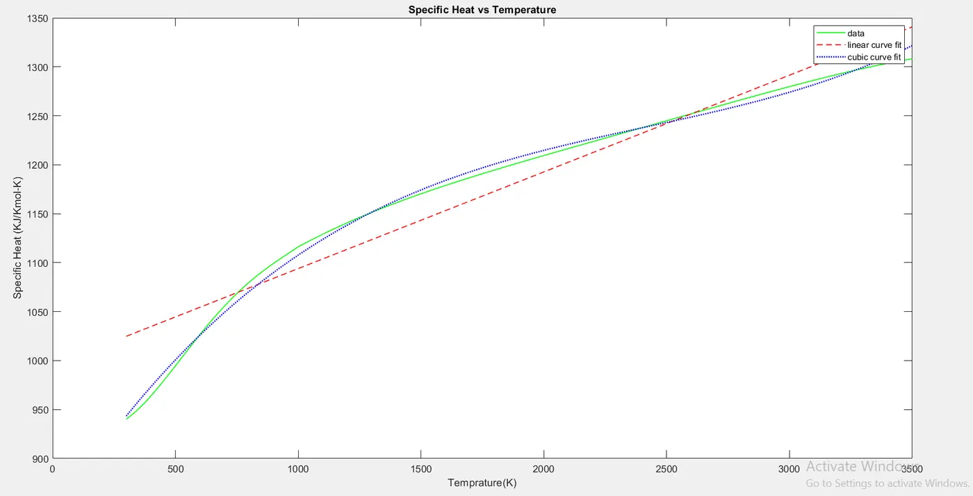
Importing the data by loading the data file and segregating the data based on dependent and independent variables. Here temperature is independent and specific heat is a dependent variable. A linear and cubic function is formulated and the coefficients of the function are formed using the polyfit function.
Based on the coefficients and independent variable is used the polyval function is used to return the corresponding values of the polynomial.
%Importing the data
cp_data=load('data_o2_cp');
temperature=cp_data(:,1);
cp=cp_data(:,2);

%Curve fit
%equation for liner curve cp=at+c
coef1=polyfit(temperature,cp,1);
predicted_cp1=polyval(coef1,temperature);

% cubic equation for curve cp=at^3+bt^2+ct+d
coef3=polyfit(temperature,cp,3);
predicted_cp3=polyval(coef3,temperature);
Comparing the Curves
After generating the values for the assumed polynomial function the data is potted in order to get a visual interpretation and comparison of the formulated polynomial and original data.
%comparing the  my curve fit with the original data
figure(1)
plot(temperature,cp,'linewidth',1,'color','g');
xlabel('Temprature(K)');
ylabel('Specific Heat (KJ/Kmol-K)');
hold on;
plot(temperature,predicted_cp1,'r--','linewidth',1);
plot(temperature,predicted_cp3,'b:','linewidth',1.5);
legend('data','linear curve fit','cubic curve fit');
title('Specific Heat vs Temperature');
hold off;
It is clearly evident that the cubic polynomial gave better results compared to linear, hence a cubic function is further used for the split-wise method in order to check for better results.
Finding the intervals for split-wise in order to get a better fit.
A plot of deviation between the cubic polynomial and the given dataset is generated to find the indices independent values where the curves are intersecting or the difference between the values is very less which may act as new end conditions for the split-wise function to be formed.
%from the plot it is clear that the cubic equation gives better result than linear
%hence cubic function will be used for splitwise method

% finding split intervals where our curve deviated least with 3rd degree
deviation3=cp-predicted_cp3;
figure(2)
plot(temperature,deviation3)
title('Deviation with Degree 3 vs Temperature');
%index at which the deviation in cp_predicted is close to zero
index_3=find(abs(deviation3)<1e-1,50);
Deviation of Cubic Function vs Temperature
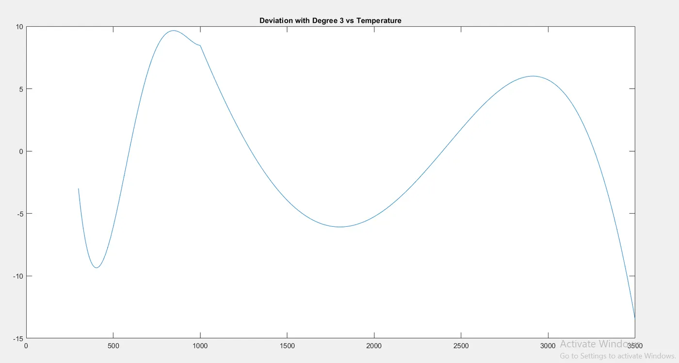
It is seen that the cubic function has 4 points where the deviation is nearly zero. the indices of the independent variable are found by using the above code where we check the difference between the values is very less and we store the indices using the find function.
Formulating the Split-Wise function and Comparing the Data
Based on the values of indices where the deviation is very less we divide the data set for independent variables in 5 Splits and generate a plot comparing the curve fit.
%we will split the curve into 5 based values from index_3
%split 1 from index 1 to 293
n3=3;
coef_sp31=polyfit(temperature(1:293),cp(1:293),n3);
predicted_sp31=polyval(coef_sp31,temperature(1:293));

%split 2 from index 294 to 994
coef_sp32=polyfit(temperature(294:994),cp(294:994),n3);
predicted_sp32=polyval(coef_sp32,temperature(294:994));

%split 3 from index 995 to 2094
coef_sp33=polyfit(temperature(995:2094),cp(995:2094),n3);
predicted_sp33=polyval(coef_sp33,temperature(995:2094));

%split 4 from index 2095 to 2997
coef_sp34=polyfit(temperature(2095:2997),cp(2095:2997),n3);
predicted_sp34=polyval(coef_sp34,temperature(2095:2997));

%split 5 from index 2998 to 3200
coef_sp35=polyfit(temperature(2998:3200),cp(2998:3200),n3);
predicted_sp35=polyval(coef_sp35,temperature(2998:3200));

predicted_sp3=[predicted_sp31;predicted_sp32;predicted_sp33;predicted_sp34;predicted_sp35];
Plot for Comparing the Curve fit
%comparing the split cibic curve fit with the original data
figure(3)
plot(temperature,cp,'linewidth',2,'color','g');
xlabel('Temprature(K)');
ylabel('Specific Heat (KJ/Kmol-K)');
hold on;
plot(temperature,predicted_sp3,'linewidth',1,'color',[0.5 0 0.5]);
legend('data','cubic split curve fit');
title('Specific Heat vs Temperature');
hold off;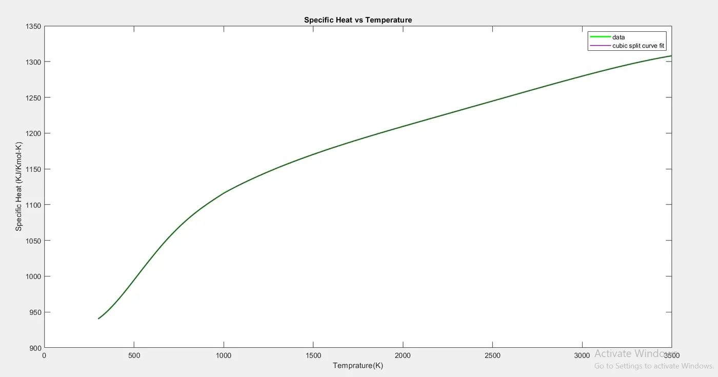
A nearly perfect fit is achieved by using the Split-Wise method.
Choose the Best Fit based on the following:-
Upon finding a curve that satisfies the data points there are 4 methods to measure the goodness of fit criteria.
The 4 methods are:-
1. The Sum of Square due to Error (SSE)
2. R-Square
3. Adjusted R-Square
4. Root Mean Square Error
The value of the above 4 methods is found using the formula explained above.
Two for loops are formed one as per the number of formulated curves and the second as per the length of the dataset.
The first for loop provides the dataset of each formulated curve one by one and in the second for loop, the data is generated to find the values for Sum of Square due to Error (SSE). Based on the value of SSE and SSR the value of R-Square is found.
%Chossing the best fit
error=zeros(3200,3);
se=zeros(3200,3);
sse=zeros(1,3);
predictedcp=[predicted_cp1 predicted_cp3 predicted_sp3];
mean_data=mean(cp);
ssr=zeros(1,3);
n=length(temperature);

for j=1:3
for i=1:3200
    error(i,j)=predictedcp(i,j)-cp(i);
    se(i,j)=error(i,j)^2;
    sse(j)=sse(j)+se(i,j);
    ssr(j)=ssr(j)+(predictedcp(i,j)-mean_data)^2;
end
end

%r square method
sst=sse+ssr;
r_sq=ssr./sst;
Similarly using the formula explained above we found the Adjusted R-Square and RMSE for the three curves. Now all the values of required for choosing the best fit is displayed in the table for easy comparison.
%adjusted r square method
%the only independent variable here is temperature
k=1;
r_sq_adj=1-(((1-r_sq.^2)*(3200-1)))./(n-1-1);

%root mean square error method (rmse)
rmse=(sse/n).^0.5;

CurveName = {'Linear Fit';'Cubic Fit';'Splitwise Cubic Fit'};
T= table(CurveName,sse',r_sq',r_sq_adj',rmse');
T.Properties.VariableNames{2} = 'SSE';
T.Properties.VariableNames{5} = 'RMSE';
T.Properties.VariableNames{3} = 'R_Square';
T.Properties.VariableNames{4} = 'R_Square_Adjusted';
The values obtained to choose the best fit for the 3 polynomial regression
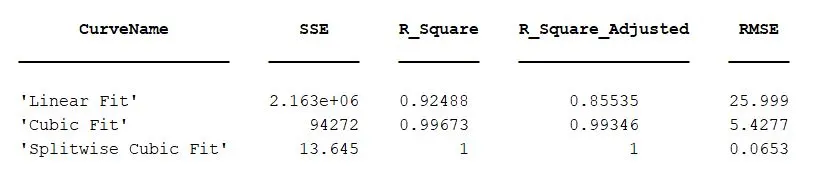
From the above table it is clear that the Splitwise Cubic Polynomial gave the best as the values of R-Square and the Adjusted R-Square is equal to 1 and the values of RMSE and SSE is minimum. Hence it solves our question of cossing the best fit.
How to fit the curve perfectly?
A curve can be made fit completely by using the following methods:-
1. Choosing the right degree of curve based on the number of points to fitted. If n is the number of points then n-1 is considered the degree of polynomial for the best fit.
2. Spliting the curve into smaller section.
3. Centering and scaling
How to get the best fit?
A perfect fit is usuallly the best fit, but a best fit can be determined using the 4 methods to measure the goodness of fit criteria.
What could be done to improve the cubic fit?
The improve the cubic fit here we used the Split-wise method. Both methods such as Split-wise and Centering and scaling can be used in order to improve the fit.
clear all;
close all;
clc

%Importing the data
cp_data=load('data_o2_cp');
temperature=cp_data(:,1);
cp=cp_data(:,2);

%Curve fit
%equation for liner curve cp=at+c
coef1=polyfit(temperature,cp,1);
predicted_cp1=polyval(coef1,temperature);

% cubic equation for curve cp=at^3+bt^2+ct+d
coef3=polyfit(temperature,cp,3);
predicted_cp3=polyval(coef3,temperature);

%comparing the  my curve fit with the original data
figure(1)
plot(temperature,cp,'linewidth',1,'color','g');
xlabel('Temprature(K)');
ylabel('Specific Heat (KJ/Kmol-K)');
hold on;
plot(temperature,predicted_cp1,'r--','linewidth',1);
plot(temperature,predicted_cp3,'b:','linewidth',1.5);
legend('data','linear curve fit','cubic curve fit');
title('Specific Heat vs Temperature');
hold off;

%from the plot it is clear that the cubic equation gives better result than linear
%hence cubic function will be used for splitwise method

% finding split intervals where our curve deviated least with 3rd degree
deviation3=cp-predicted_cp3;
figure(2)
plot(temperature,deviation3)
title('Deviation with Degree 3 vs Temperature');
%index at which the deviation in cp_predicted is close to zero
index_3=find(abs(deviation3)<1e-1,50);

%we will split the curve into 5 based values from index_3
%split 1 from index 1 to 293
n3=3;
coef_sp31=polyfit(temperature(1:293),cp(1:293),n3);
predicted_sp31=polyval(coef_sp31,temperature(1:293));

%split 2 from index 294 to 994
coef_sp32=polyfit(temperature(294:994),cp(294:994),n3);
predicted_sp32=polyval(coef_sp32,temperature(294:994));

%split 3 from index 995 to 2094
coef_sp33=polyfit(temperature(995:2094),cp(995:2094),n3);
predicted_sp33=polyval(coef_sp33,temperature(995:2094));

%split 4 from index 2095 to 2997
coef_sp34=polyfit(temperature(2095:2997),cp(2095:2997),n3);
predicted_sp34=polyval(coef_sp34,temperature(2095:2997));

%split 5 from index 2998 to 3200
coef_sp35=polyfit(temperature(2998:3200),cp(2998:3200),n3);
predicted_sp35=polyval(coef_sp35,temperature(2998:3200));

predicted_sp3=[predicted_sp31;predicted_sp32;predicted_sp33;predicted_sp34;predicted_sp35];

%comparing the split cibic curve fit with the original data
figure(3)
plot(temperature,cp,'linewidth',2,'color','g');
xlabel('Temprature(K)');
ylabel('Specific Heat (KJ/Kmol-K)');
hold on;
plot(temperature,predicted_sp3,'linewidth',1,'color',[0.5 0 0.5]);
legend('data','cubic split curve fit');
title('Specific Heat vs Temperature');
hold off;

%Chossing the best fit
error=zeros(3200,3);
se=zeros(3200,3);
sse=zeros(1,3);
predictedcp=[predicted_cp1 predicted_cp3 predicted_sp3];
mean_data=mean(cp);
ssr=zeros(1,3);
n=length(temperature);

for j=1:3
for i=1:3200
    error(i,j)=predictedcp(i,j)-cp(i);
    se(i,j)=error(i,j)^2;
    sse(j)=sse(j)+se(i,j);
    ssr(j)=ssr(j)+(predictedcp(i,j)-mean_data)^2;
end
end

%r square method
sst=sse+ssr;
r_sq=ssr./sst;

%adjusted r square method
%the only independent variable here is temperature
k=1;
r_sq_adj=1-(((1-r_sq.^2)*(3200-1)))./(n-1-1);

%root mean square error method (rmse)
rmse=(sse/n).^0.5;

CurveName = {'Linear Fit';'Cubic Fit';'Splitwise Cubic Fit'};
T= table(CurveName,sse',r_sq',r_sq_adj',rmse');
T.Properties.VariableNames{2} = 'SSE';
T.Properties.VariableNames{5} = 'RMSE';
T.Properties.VariableNames{3} = 'R_Square';
T.Properties.VariableNames{4} = 'R_Square_Adjusted';