Curve Fit In MATLAB

Aim - To write a code to show a curve fit on a data .

Objective –

1. Plot the linear and cubic fit curves along with the raw data point.

1. Write a code to show split wise method.

3. Explain the parameters used to measure the fitness characteristics

Introduction -

Curve fitting is the process of constructing a curve , or mathematical function which best represents the real series of data . It is highly effective in mathematical model of real process .

There are two types of curve fit , best and perfect . We will be using best fit which is obtained by increasing the degree of the polynomial or using split wise method .Sometimes we may get perfect fit using the split wise method .

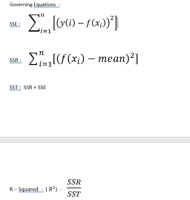
The goodness of the fit is decided by 4 process .

1. SUM OF SQUARED ERRORS .
2. R- SQUARE ADJUSTED
3. R – SQUARE
4. ROOT MEAN SQUARE .

R-square value always remains between 0 and 1 .

If R- square value is below 0.95 – Bad fit

If R- square value is equal to 0.95 – good fit

If R- square value is above 0.95 – Best fit

If R- square value is 1 – perfect fit

Code :

clc
clear all
close all

% writting the data to a variable 
cp_data  = load ('data') ; % contains data temp and specific heat .
Temp = cp_data(:,1);  % x axis values ..
cp = cp_data(:,2) ;    % y axis values ..


% curvefit..........

% Two degree polynomial fit ....
coe_efficient = polyfit(Temp,cp,2);
predict_cp_1 = polyval(coe_efficient , Temp ) ;    


% Three degree curve fit ... 
% s = error estimating structure  
% m = centering and scalling values
% used to improve the cubic or higher order polynomial fit ......

[coe_efficient_2,s,m] = polyfit(Temp,cp,3);
predict_cp_2 = polyval(coe_efficient_2 , Temp,s,m ) ;    


% split wise  curve fit Method ........>
% spliting the data in 8 equal parts 
%..........
a = 1;
n = 400 ; 
% A loop is used to get the data from the 8 equal parts in which the data
% was devided ...........
for i = 1 : 8
 
    coe_efficient_3 = polyfit(Temp(a:n),cp(a:n),2);
    predict_cp_3(a:n,1)  = polyval(coe_efficient_3 , Temp(a:n) ) ;   
    
    a = n+1 ;
    n= n+400 ;
      
end

%Plotting the curve fit .....>
%plot......

hold on ;
grid on ;
plot(Temp , cp ,'r --','linewidth',2.5);
plot (Temp ,predict_cp_1 , 'b','linewidth',1.5);
plot( Temp , predict_cp_2 , 'y','linewidth',1.5);
xlabel('Temparature' );
ylabel('Specific heat ' );
legend ('original data ','quadratic ploynomial ','cubic ploynomial');


% split wise Method  plot ........>

figure(2) 
hold on ;
grid on ;
plot(Temp , cp ,'r --','linewidth',3);
plot(Temp ,predict_cp_3,'b','linewidth',1.5  ) ;
xlabel('Temparature' );
ylabel('Specific heat ' );
legend ('original data ' ,'split curve ' );
title('Split Wise curve fit ');

% error estimation ...
% best fit ....estimation to all three type of curve fit ....

mean = sum(cp)/length(cp) ;  % mean from original  data .... 

% SSR -  sum of square of regression ...
ssr1 = sum( (predict_cp_1 - mean ).^2);
ssr2 = sum( (predict_cp_2 - mean ).^2);
ssr3 = sum( (predict_cp_3 - mean ).^2);

% SSE - sum of squared error ....
sse1 = sum((cp - predict_cp_1).^2) ;
sse2 = sum((cp - predict_cp_2).^2) ;
sse3 = sum((cp - predict_cp_3).^2) ;

% SST - total sum of squares .....
sst1 = ssr1 +sse1 ; 
sst2 = ssr2 +sse2 ;
sst3 = ssr3 +sse3 ;

% R - square ....the final result for best fit .....
%Displayed in the command window ........
r_square_1 = ssr1/sst1 
r_square_2 = ssr2/sst2 
r_square_3 = ssr3/sst3 

Explanation

1. The first three lines of the code are used to refresh the command window .
2. The file containg the data is stored in the same location where all the matlab files are present .
3. It is now loaded into matlab using a variable " cp_data " .
4. Now the x and y values are written to variables so that they could be accesed .
5. Now to represent the Two degree polynomial , the ployval and plyfit commands are used .
6. They calculate the co-efficients of the second degree polynomial and using polyfit command finds the best points to represent the data .
7. After this same commands are used for a three degree cubic polyomial . But an error regarding the scaling would be seen . This is corrected using two more variables "s " and "m" . They represent the error in the structures and other contains scaling vaules .
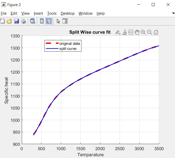
8. After this split wise method is used to represent the data more correctly .
9. The data has been divided into 8 equal parts .
10. A for loop is used to predict the values from each part of the data .
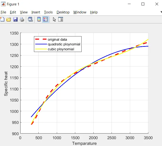
11. Now after getting all the values the plot is drawn with original data .
12. A plot for split wise method is also shown .
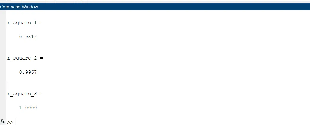
13. After plotting the R-Squared values of all the three curve fit plots are determined .
14. The value of R-squared shows which curve fit is best or perfect fit to the original data .

Errors seen -

The above error was corrected using the following command %....>

% Three degree curve fit ... 
% s = error estimating structure  
% m = centering and scalling values
% used to improve the cubic or higher order polynomial fit ......

[coe_efficient_2,s,m] = polyfit(Temp,cp,3);
predict_cp_2 = polyval(coe_efficient_2 , Temp,s,m ) ;    

Results From abve plots : -

Thus from above above figure we can say that ,

1. The Quadratic polynomial is a Good fit for the data
2. The Cubic polynomial is a Good fit for the data .
3. The curve fit using the split wise method gave a perfect fit .

Conclusion

All the objectives have been completed successfully from the above code .

reference :

https://www.statisticshowto.com/curve-fitting/

https://statisticsbyjim.com/regression/curve-fitting-linear-nonlinear-regression/

Thank You .