P-V DIAGRAM FOR OTTO CYCLE

Aim - To write a code to plot a P-V diagram for otto cycle .

Objective -

1 . P – V diagram

2. Thermal Efficiency of Otto cycle .

Introduction -

An Otto cycle is an idealized thermodynamic cycle that describes the functioning of a typical spark engine . It is the thermodynamic cycle most commonly found in automobile engines.

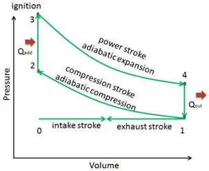
Otto cycle Process –

1. Isentropic Compression - From state 1 to state 2 .
2. Isochoric Compression - From state 2 to state 3 .
3. Isentropic Expansion - From state 3 to state 4 .
4. Isochoric Expansion - From state 4 to state 1 .

Governing Equations

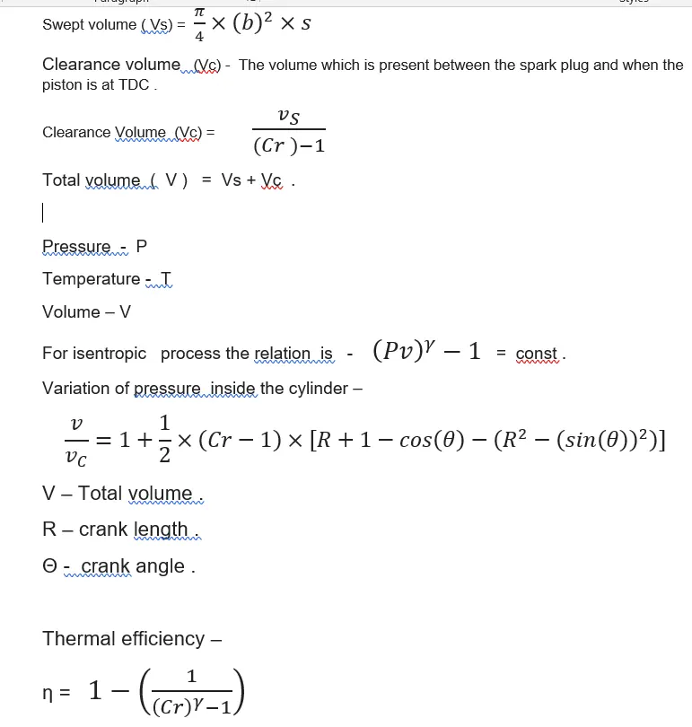
Bore (b) – dia of the piston .

Stroke (s) – distance travelled from TDC to BDC .

Connect_rod - The rod that creates link between piston and crankshaft .

Swept volume – The volume that it has from TDC to BDC .

Cr - Compression ratio .

Code -

clear all
close all
clc

% inputs 
gamma = 1.2;
t3 = 2300 ;

%  state variables 
p1 = 101325 ;
t1 = 500 ;

% engine parameters 
bore = 0.1 ;
stroke_1 = 0.1 ;
connect_rod =  0.15 ;
cr = 12 ;


% calculating swept volume and total volume 
V_swept =(pi/4)*bore^2*stroke_1 ;
V_clearence = V_swept/(cr-1) ;

v1 = V_swept +  V_clearence; 
v2 =  V_clearence; 

% state variable for 2 
%p2v2^gamma = p1v1^2gamma 
p2 = p1*cr^gamma ;

% using idel gas law 
%p1v1/t1 =p2v2/t2
t2 = p2*v2*t1/(p1*v1);

con_c = p1*v1^gamma;
V_comp =  engine_kinematics (bore , stroke_1 , connect_rod , cr , 180 ,0 ) ;
                           
p_comp = con_c./(V_comp).^gamma ;





%state variables at state point 3 
v3 = v2 ;
% pressure at 3 using ideal gas law 
p3 = (p2*t3)/t2 ;



con_A =  p3*v3^gamma;
V_expan =  engine_kinematics (bore , stroke_1 , connect_rod , cr , 0, 180 ) ;
                           
p_expan = con_A./V_expan.^gamma ;


% state variables at point 4 
v4 = v1 ;
p4 =p3*(v3/v4)^gamma ;


figure(1)
grid on ;
hold on ;
plot(v1,p1,'*','color','g');
plot(V_comp,p_comp,'color','r');
plot(v2,p2,'*','color','g');
plot([v2 v3],[p2 p3],'color','b');
plot(v3,p3,'*','color','g');
plot(V_expan,p_expan,'color','r');
plot(v4,p4,'*','color','g');
plot([v4 v1],[p4 p1],'color','b');



thermal_efficiency = 1 - (1 /(cr^(gamma-1))) 

Function - engine kinematics

function [V] = engine_kinematics ( bore , stroke_1, connect_rod , cr,start_crnk,end_crnk )

% engine parameters 

c = (stroke_1)/ 2 ; 
R = connect_rod/c ;


V_s =(pi/4)*(bore)^2*stroke_1 ;
V_c = V_s/(cr-1); 


theta  = linspace(start_crnk,end_crnk,200) ;


term1 = 0.5*(cr-1) ;
term2 = R + 1 - cosd(theta);
term3 = (R^2 - sind(theta).^2).^0.5 ;


V = (1+ term1*(term2-term3)).*V_c; 


end 

Explanation -

1. First three lines are the clear all , close all , clc to update and clean the workspace .
2. The assumed values are then defined in the programe .
3. The engine parameters are also defined to calculate the "engine kinematics" .
4. The total volume and the swept volume is calculated using the equations written before .
5. The state variables for state 2 is calculated which are "p2 and t2 " using the state one variables using the equations .
6. Now the position os the state 2 is obtained but to obtain the path that the volume and pressure follows is calculated using "engine_kinematics" function .
7. The function calculates the volume that is changing till state 2 Which is "V_compression " and also the P_compression ' is calculated . This is govereng mainly by the crank angle which go from "180 - 0 " . All the prameters are also passed to it .
8. The above Preocess is now repeated from state 3 to state 4 with crank angle from "0 - 180 " . The function now calculates "V_expansion " and "P_expansion " .
9. After caculating all the state points it is then plotted using plot command .
10. The required graph is formed .

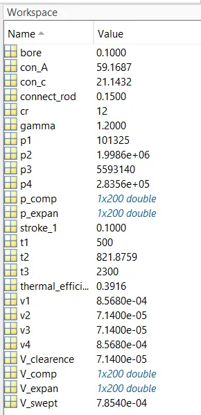
The values in the Variables are -

The P-V Plot -

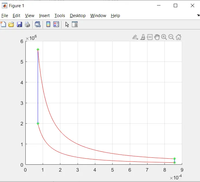
The Thermal Efficiency is obtained as 39 % .

Conclusion -

The P-V diagram is obtained and the efficiency is also calculated .

Thank You .