Conjugate Heat Transfer Analysis on a graphics card.
Conjugate Heat Transfer Analysis of a Graphics Card
Aim
To carry out the Conjugate Heat Transfer(CHT) Analysis on a graphics card at various velocities of the cooling fluid and to compare the cooling effect on the processor. Also, to identify the potential hotspots in the model.
Introduction
Conjugate Heat Transfer(CHT) is the heat transfer between the solid and fluid domains by exchanging thermal energy at their interfaces in contact.
A graphics card, also known as video card is installed in most computing devices to display the graphic content with high clarity, definition, colour and appearance. These graphics are present in almost all modern-day computers and high processing computers. They have their own in-built memory and cooling system.
The need for a cooling system is for the reason that all electronics drop their efficiencies when they get over-heated and the processor in these graphic cards is no different. It generates a lot of heat and has to be evacuated in order to proper working of the graphic processing unit. A cooling fan is used to dissipate the heat and the configurations of these fans and design optimisation can be decided with the help of a CHT analysis.
The simulation also helps in visualising the effects of the coolant air at different velocities and to choose the best practical velocity for the real-world application.
Solving methodology and modelling approach
The solution will be carried out for three different velocities, but the model remains unchanged in all these simulations.
The simulation is carried out for 1m/s, 3m/s and 5m/s respectively.
Since the model, pre-processor settings and the some physics remain unchanged throughout the course of 3 simulations, it will be mentioned only once.
Common Setup
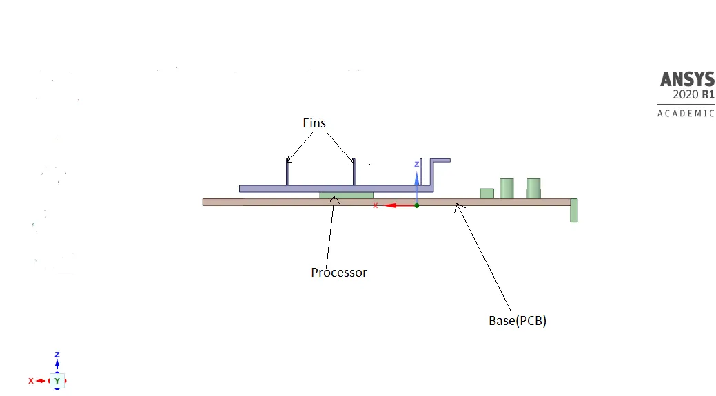
The CAD model provided has mainly 3 solid components namely the fins, the processor and the PCB base. The model is also provided with an enclosure to facilitate as the fluid domain in the simulation.
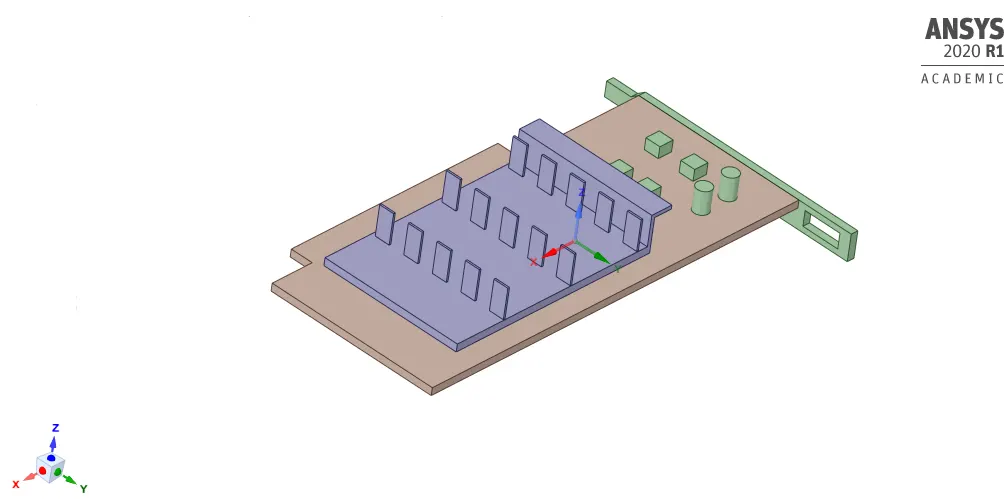
The parts of the model are named below in the side view.
This model is provided with an enclosure to facilitate the flow of fluid.
Once the model is ready, it is processed for meshing with refinements wherever required. The below picture denotes the meshed enclosure, containing the model.
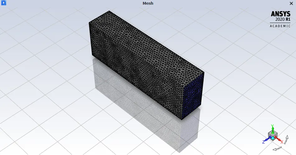
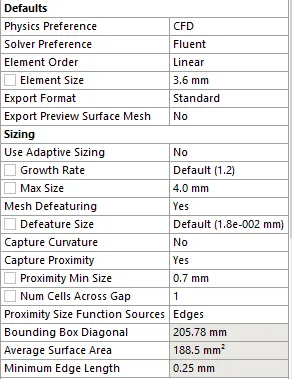
The enclosure in the picture was meshed with a global mesh size of 3.6mm and also the proximity was captured wherever the model had smaller features with the minimum mesh size cap at 0.7mm. The picture of the mesh setting is given below.
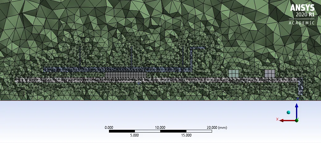
The picture below shows the section plane of the model at the centre and the variation of mesh at different regions.
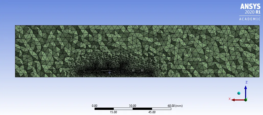
In any heat transfer simulation, for the heat to dissipate properly, it is very essential for the mesh to be conformal at various surfaces. The picture below clarifies that the need for a conformal mesh is fulfilled.
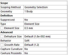
Apart from the global mesh sizing, the processor was meshed with a finer mesh size to efficiently capture the heat generated and to dissipate it accordingly. The element size used was 0.5mm.
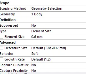
Similar to the processor, the fins also play a vital role in heat dissipation and it is essential to capture it efficiently. Hence, the body sizing method, with a mesh size of 0.6mm is used keeping all other properties as default.
The body sizing mesh method was also used on the base of the model. The element size used was 6mm in order to facilitate the smooth growth of mesh size from the processor to the enclosure.
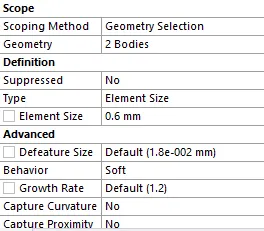
The final property, which is as important as the refinement of the mesh is the quality of the elements or cell volumes. Considering the academic limit of 512000 cells, after the refinements, a pretty good average element quality of 83.335% was achieved.
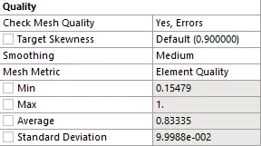
The element quality mesh metric is shown below and the majority of elements have achieved a good element quality.
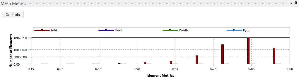
The mesh contains 103532 modes and 511165 elements which is just below the maximum academic limit.

Solver Physics
A pressure-based steady-state simulation is set since the flow velocity is low and also the solution is concentrated on the result at the end rather than at intervals.
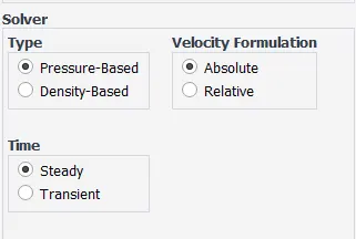
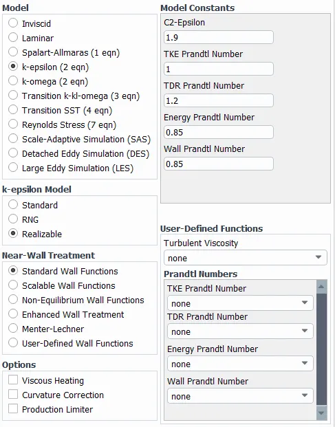
Since the solution doesn't worry about the pressure gradient, the Realizable k-epsilon turbulence model with standard wall functions is used which is more appropriate and optimized for flows near boundaries.
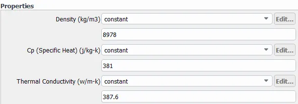
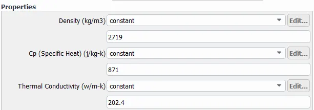
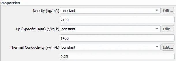
As for the materials used, the processor is made of copper, aluminium fins and the base is made of a glass-reinforced epoxy laminate material called FR-4. Air is used as the circulating coolant inside the chamber or enclosure.
The properties of copper are as follows(fluent database)
The properties of Aluminium are as follows(Fluent database)
The properties of FR-4 were not readily available in the database. Hence, it was referred from external sources.
Since most graphics cards are air-cooled, it is used as the cooling fluid and the default properties in the fluent database are used.
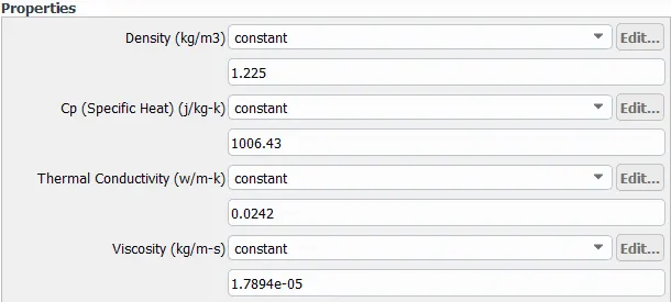
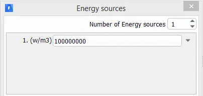
The processor is the power-house and meanwhile, generates a lot of heat and this heat generated is provided as the heat source.
The dimensions of the processor are 0.008m in length,0.008m in breadth and 0.001m in thickness.
The processor power is considered to be 6.4W(single heat source).
The heat generated by the processor(in `W/m^3`)=(Power/Volume)
`=>``(6.4/((0.008)(0.008)(0.001)))`
`=1`*`10^8``W/m^3`
The same is shown below
Once these properties are set, the solution is initialised using hybrid initialization with suitable plots, contours and animation.
The simulation was run at three different velocities of air namely case 1, case 2 and case 3 respectively.
Case 1
The inlet velocity of air= 1m/s (along negative x-axis)
The inlet temperature of air= 300 K
The outlet pressure of air will be at 0(zero) gauge pressure(1 atm).
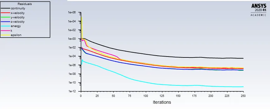
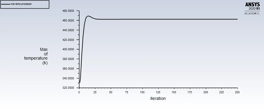
The solution ran for around 250 iterations and the residuals seemed to be stable. Also, the heat transfer coefficient and the maximum temperature attained also remained constant at this stage and hence it was evident that the solution got converged.
The residual plot is shown below
The heat transfer coefficient achieved by the processor is 691.7`W/(m^2K)`.
The maximum temperature observed was 462.3 K and it is clearly seen in the temperature contour below.
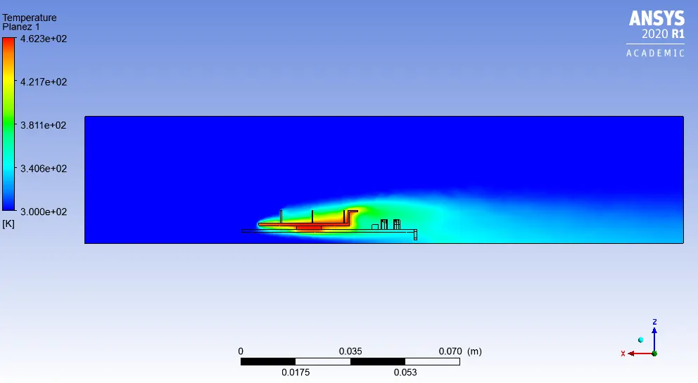
The maximum temperature thus seen is achieved by the processor which is shown in the below plot of the area-weighted average of the heat fluxes in the processor.
The animation of the temperature contour, developing for a flow of 1m/s can be viewed using the link https://drive.google.com/file/d/1e2F3HQIVtLxn-juXK_BDWqEc1DxIPK_k/view?usp=sharing
Case 2
The inlet velocity of air= 3m/s (along negative x-axis)
The inlet temperature of air= 300 K
The outlet pressure of air will be at 0(zero) gauge pressure(1 atm).
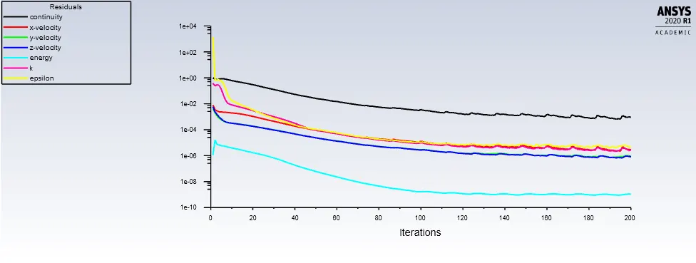
The solution ran for around 200 iterations and the residuals seemed to be stable. Also, the heat transfer coefficient and the maximum temperature attained also remained constant at this stage and hence it was evident that the solution got converged.
The residual plot is shown below
The heat transfer coefficient achieved by the processor is 828.44`W/(m^2K)`.
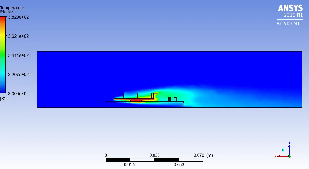
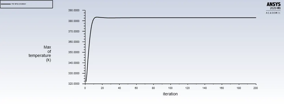
The maximum temperature observed was 383.4 K and it is clearly seen in the temperature contour below.
The maximum temperature thus seen is achieved by the processor which is shown in the below plot of the area-weighted average of the heat fluxes in the processor.
The animation of the temperature contour, developing for a flow of 3m/s can be viewed using the link https://drive.google.com/file/d/1ICFieYoli921VPEsqpOev2gdeR9wy9p3/view?usp=sharing
Case 3
The inlet velocity of air= 5m/s (along negative x-axis)
The inlet temperature of air= 300 K
The outlet pressure of air will be at 0(zero) gauge pressure(1 atm).
The solution ran for around 200 iterations and the residuals seemed to be stable. Also, the heat transfer coefficient and the maximum temperature attained also remained constant at this stage and hence it was evident that the solution got converged.
The residual plot is shown below
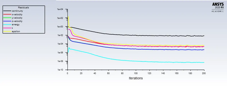
The heat transfer coefficient achieved by the processor is 1049.7`W/(m^2K)`.
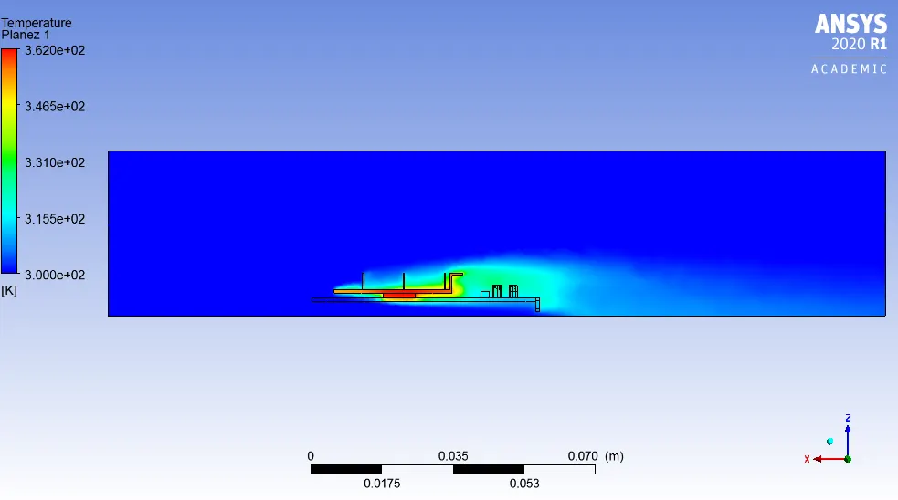
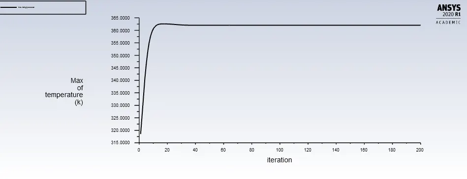
The maximum temperature observed was 362 K and it is clearly seen in the temperature contour below.
The maximum temperature thus seen is achieved by the processor which is shown in the below plot of the area-weighted average of the heat fluxes in the processor.
The animation of the temperature contour, developing for a flow of 5m/s can be viewed using the link https://drive.google.com/file/d/1DuKhnYGjrTp9sOvhGmasMxkQSRdK4Mue/view?usp=sharing
Comparison
| Velocity`(m/s)` | Heat Transfer Coefficient`(W/(m^2K))` | Maximum Temperature`(K)` |
| 1 | 691.7 | 462.3 |
| 3 | 828.44 | 383.4 |
| 5 | 1049.7 | 362 |
From the above table, it is clear that the case with the velocity of 5m/s has the highest Heat transfer coefficient and the lowest temperature. In contrast, the case with the velocity of 1m/s has the least Heat transfer coefficient and the highest temperature.
Conclusion
The velocity of 5m/s is able to dissipate the heat more than that of 3m/s and 1m/s. The processor is maintained at a much lower temperature because it is able to achieve the highest heat transfer coefficient among the three cases.
The processor and the fin are the potential hotspots because one of their sides(the side opposite to the flow of air) doesn't get exposed to a lot of air since the air gets expanded and forms a negative velocity in that region, and hence it is possible to have insufficient heat dissipation in the region, thus forming hot pockets.