Challenge on Combustion
Introduction
A combustor, which is also known as a burner, combustion chamber, the flame holder is a component of a gas turbine or any engine where combustion takes place. There are a variety of combustors used for various purposes.
The main characteristics that are concentrated while designing the combustor are the power output, efficiency, emissions etc.
Combustion can be classified based on various characteristics. One such category is based on the mixing of fuel and air.
- Based on mixing
- Non-premixed combustion
- Pre-mixed combustion
- Partially premixed combustion
As mentioned earlier, emissions are one of the most important characteristics in fossil fuel combustors due to the adverse effects on the environment and stringent government norms.
Modelling and Solving approach
In this simulation, we carry out the combustion in a cylindrical non-premixed combustor, and we mainly focus on the emissions caused by the combustion and work towards minimizing them considerably.
Due to hardware and software limitations, we simulate one slice of the cylindrical model. This approach is suitable since the model is axisymmetric.
We use Fick's law of dilute approximation which takes into account the turbulent diffusion and not the laminar diffusion. This is done since the laminar diffusion is negligible compared to the turbulent diffusion. Here, we check the diffusion of one species in the entire mixture of species rather than checking the diffusion in the presence of individual species.
To calculate the combustion source, we use the Finite rate Eddy dissipation model. It is the combination of Finite Rate chemistry and Eddy dissipation model. In Finite rate chemistry, we solve the Ordinary Differential Equations to calculate the rate of production of all the species. Whereas in Eddy dissipation model, the simulation is approximated to some definite values of the terms k and `epsi` of the transport equation and once those values are achieved, the mixture is burnt instantaneously.
Hence, the Finite Rate Eddy dissipation model combines both Finite Rate Chemistry and Eddy dissipation models to trade-off the limitations that they possess individually.
Preprocessor and Solver Setup
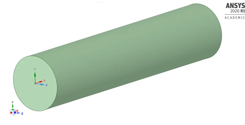
The model consists of a cylinder with the fuel inlet at the centre and surrounded by air inlet. It is shown below. The fuel inlet is situated at the origin of the model.
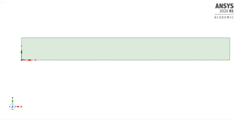
Due to limitations in hardware and the academic version of Ansys, the simulation is carried out on a slice of the entire axisymmetric geometry. The 2D model is shown below. The length of the model along the X-axis is 791.82mm with the fuel inlet being 1.6526mm and the air inlet being 82.645mm. The outlet is 85.1958mm in length.
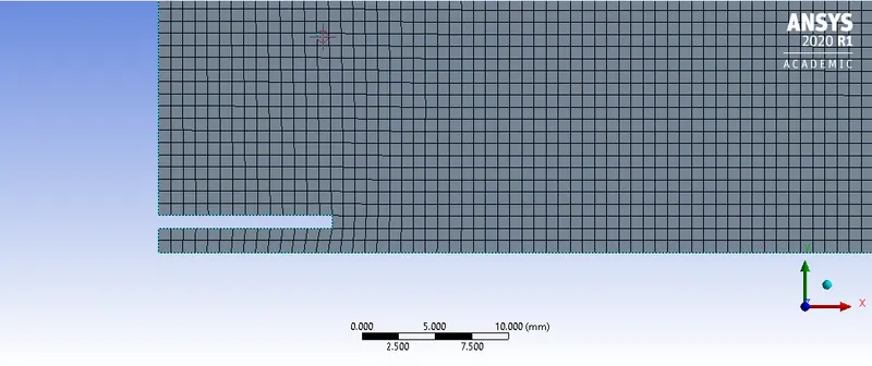
Due to the simplicity of the geometry, an all quad mesh could be achieved. A mesh size of 0.825mm was used throughout the geometry. The picture of the mesh near the inlet is shown below.
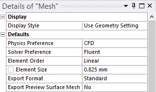
At this mesh size, 99944 nodes and 98866 elements were formed.

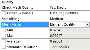
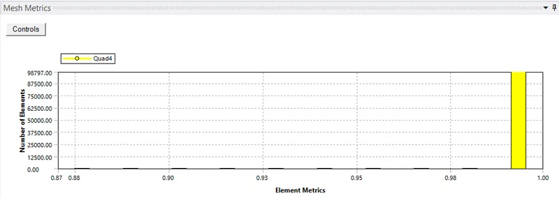
A very good mesh quality was achieved with an average of 99.883% element quality.
While setting up the solver, a pressure-based solver was used and since one slice of the cylinder was used for simulation, an axisymmetric case is set up.
A standard 2 equation k-epsilon viscous model was used with standard wall treatment.
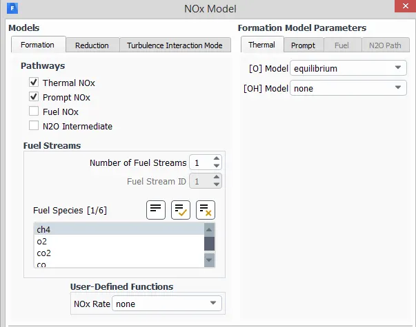
An eddy dissipation species transport equation in the presence of NOx and Soot models.
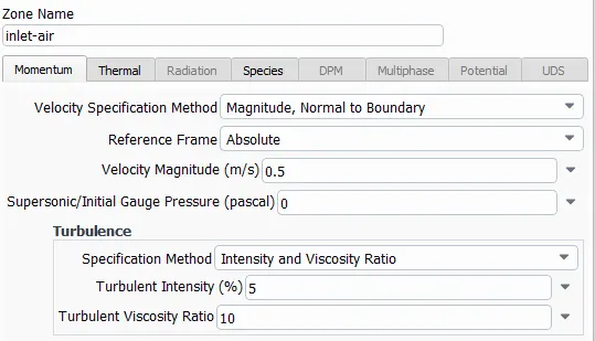
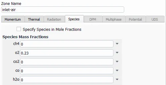
The air is let in with a velocity of 0.5m/s at a temperature of 300K with the concentration of O2 being 0.23 by mass.
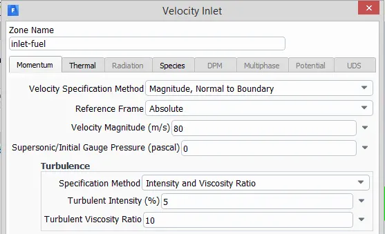
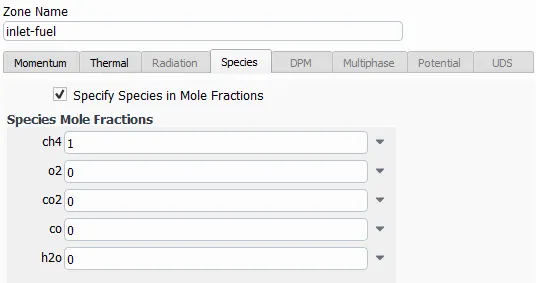
The fuel is let in with a velocity of 80m/s and with varying concentrations for different cases and hence will be discussed individually.
Since we are checking for the pollutants, contours of CO2, NO, Soot along with the contours of CH4 are included.
An animation of the contours of Static Temperature is also included and initialised using hybrid initialisation. The simulation is run for 500 iterations, which seems converged way before reaching the 500 iteration mark.
During the post-processing of the results, several line probes were used at various locations of the model. They are at distances of 10mm, 25mm, 40mm, 55mm, 70mm, 100mm, 150mm, 250mm, 350mm, 400mm, 450mm, 475mm, 500mm, 525mm, 550mm, 575mm, 600mm and 700mm from the inlet or the origin. 25 samples were used from each of the lines.
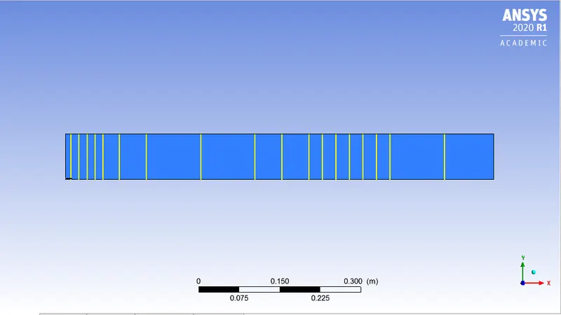
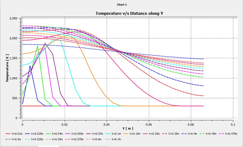
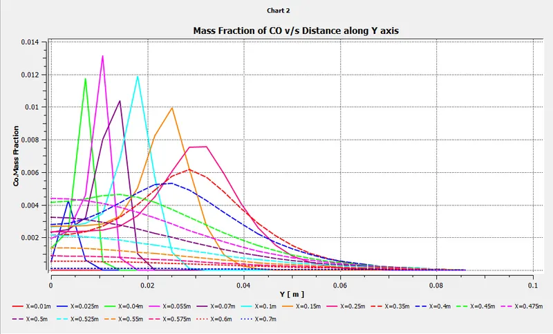
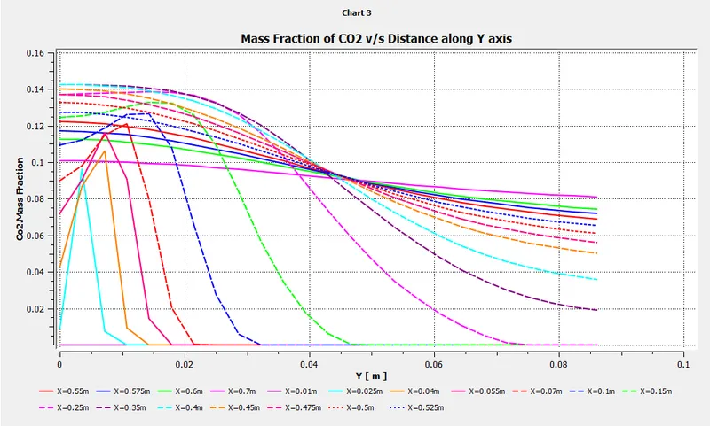
Several charts were plotted for each of the cases, which include Mass fraction of CO(Carbon Monoxide) v/s distance along the Y axis, Mass fraction of CO2(Carbon Dioxide) v/s distance along Y-axis, Mass fraction of NO(Oxides of Nitrogen) v/s distance along Y-axis, Mass fraction of Soot v/s distance along Y-axis and Mass fraction of temperature v/s distance along Y-axis.
Case 1: 100% CH4
In this case, the fuel having CH4(methane) entirely is used.
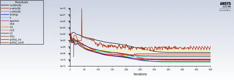
The solution is then run for 500 iterations with the setup mentioned above. The scaled residuals are shown below and it quite evident that the solution is converged.
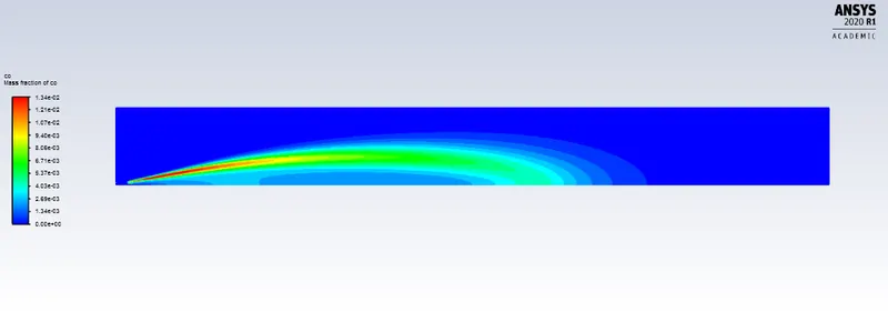
The contour of the mass fraction of CO is shown below.
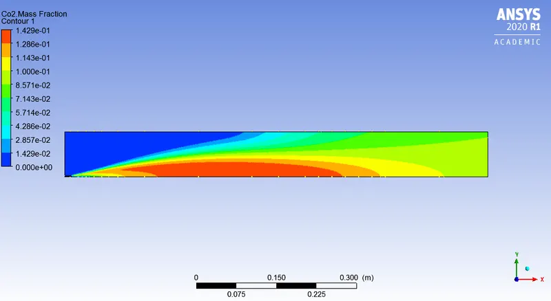
The contour of the mass fraction of CO2 is shown below.
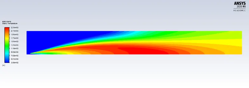
The contour of the temperature is shown below. The peak temperature attained is 2310K.
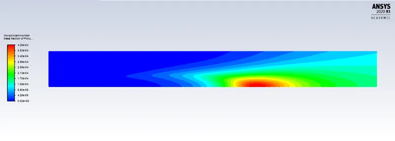
The contour of the mass fraction of the pollutant NO is shown below.
The chart for the change in Temperature along the Y-axis at various lines along X-axis is shown below.
The chart for the change in the mass fraction of Carbon Monoxide along the Y-axis at various lines along X-axis is shown below.
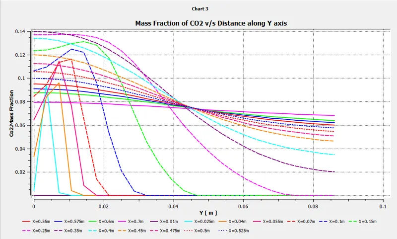
The chart for the change in the mass fraction of Carbon Dioxide along the Y-axis at various lines along X-axis is shown below.
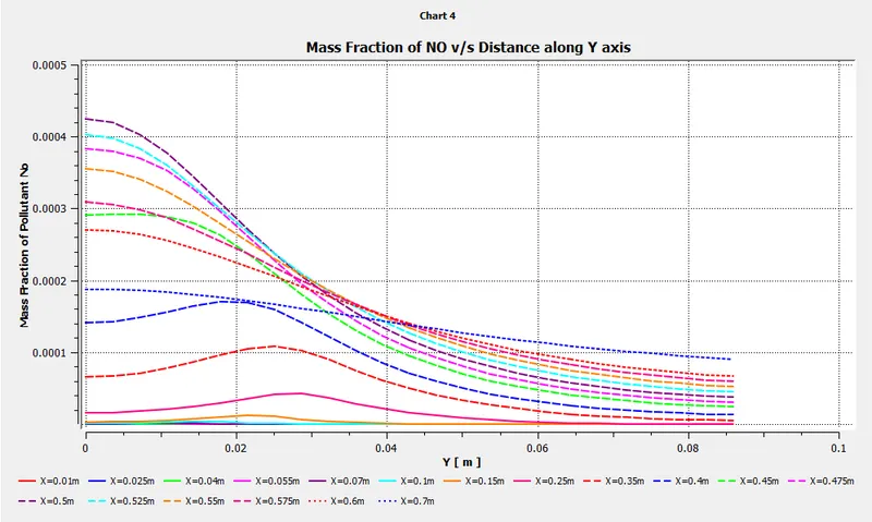
The chart for the change in the mass fraction of the oxides of Nitrogen along the Y-axis at various lines along X-axis is shown below.
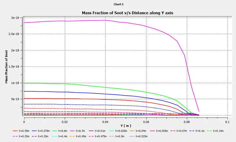
The chart for the change in the Mass fraction of Soot along the Y-axis at various lines along X-axis is shown below.
The animation of the Temperature contour can be accessed using the link https://drive.google.com/file/d/12ck6QArmp-ZgQr-leI6pv_3jmQAzuDQZ/view?usp=sharing
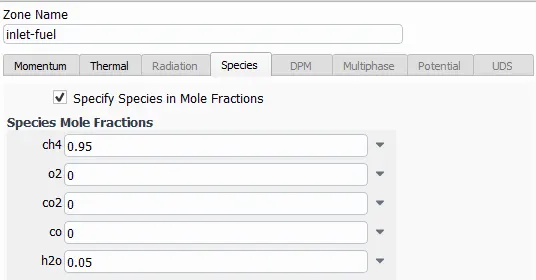
Case 2: 95% CH4 and 5% water(H2O)
Here, 5% of water by mole fraction is added to study the change is results.
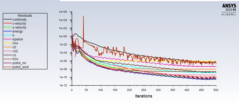
The solution is then run for 500 iterations with the setup mentioned above. The scaled residuals are shown below and it quite evident that the solution is converged.
The contour of the mass fraction of CO is shown below.
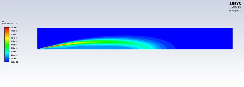
The contour of the mass fraction of CO2 is shown below.
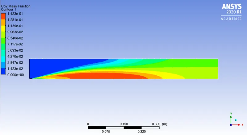
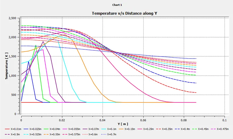
The contour of the temperature is shown below. The peak temperature attained is 2300K.
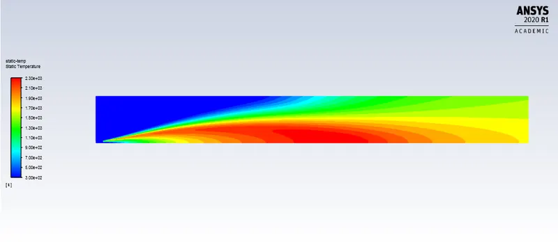
The contour of the mass fraction of the pollutant NO is shown below.
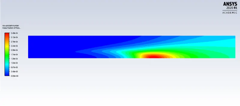
The chart for the change in Temperature along the Y-axis at various lines along X-axis is shown below.
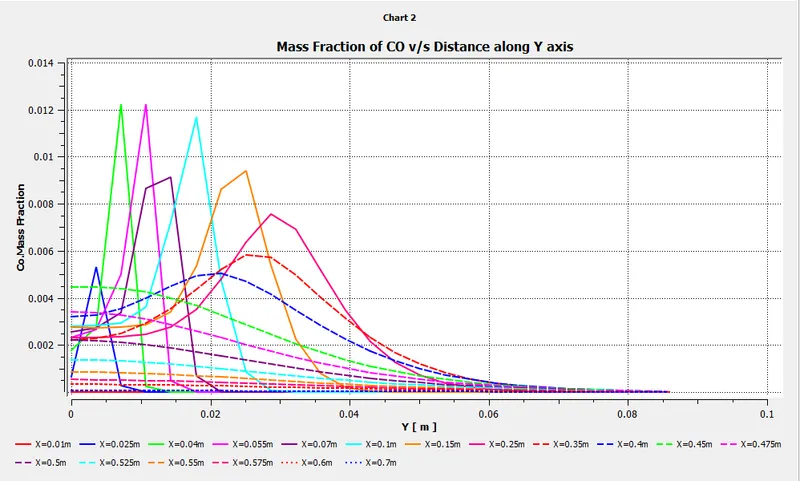
The chart for the change in the mass fraction of Carbon Monoxide along the Y-axis at various lines along X-axis is shown below.
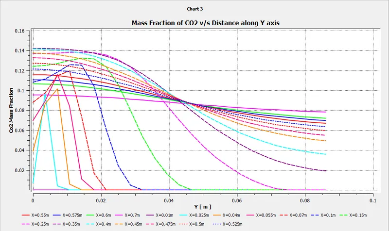
The chart for the change in the mass fraction of Carbon Dioxide along the Y-axis at various lines along X-axis is shown below.
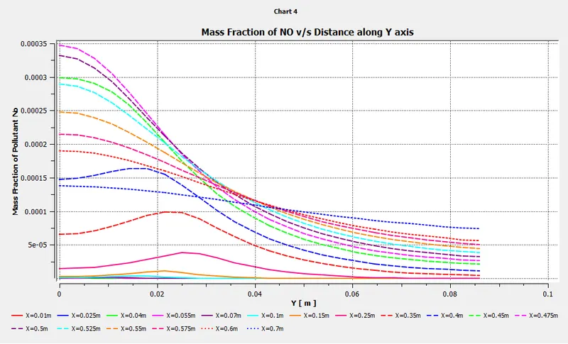
The chart for the change in the mass fraction of the oxides of Nitrogen along the Y-axis at various lines along X-axis is shown below.
The chart for the change in the Mass fraction of Soot along the Y-axis at various lines along X-axis is shown below.
The animation of the Temperature contour can be accessed using the link https://drive.google.com/file/d/1CQXCHj1wQnoiul8RUAYY8KHXLXxx6sej/view?usp=sharing
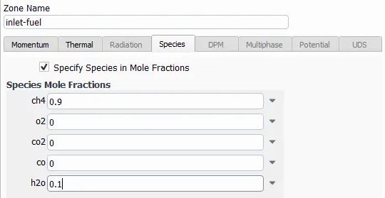
Case 3: 90% CH4 and 10% water(H2O)
Here, 10% of water by mole fraction is added to study the change is results.
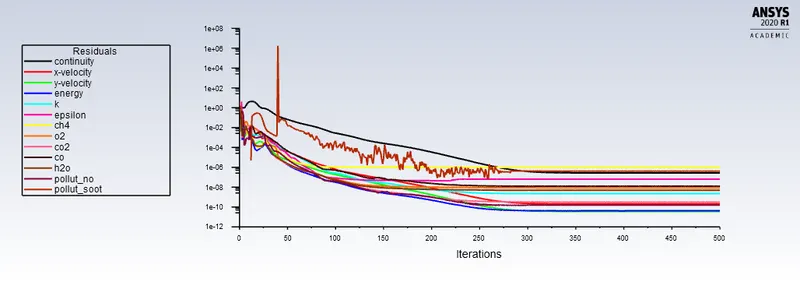
The solution is then run for 500 iterations with the setup mentioned above. The scaled residuals are shown below and it quite evident that the solution is converged.
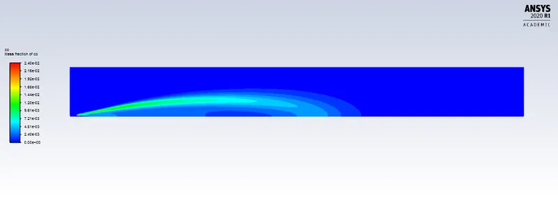
The contour of the mass fraction of CO is shown below.
The contour of the mass fraction of CO2 is shown below.
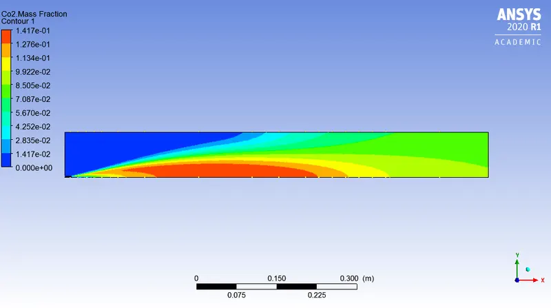
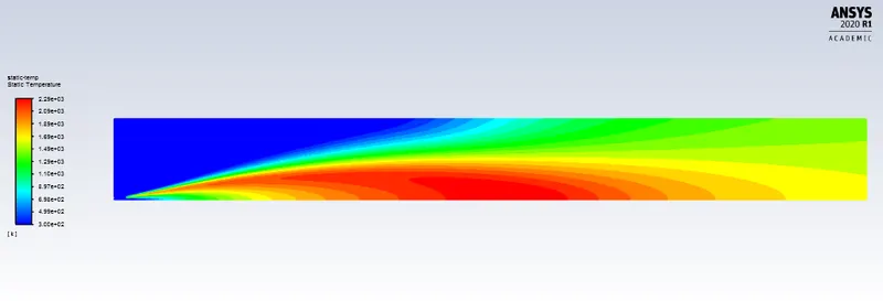
The contour of the temperature is shown below. The peak temperature attained is 2290 K.
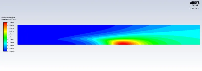
The contour of the mass fraction of the pollutant NO is shown below.
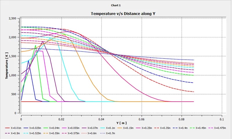
The chart for the change in Temperature along the Y-axis at various lines along X-axis is shown below.
The chart for the change in the mass fraction of Carbon Monoxide along the Y-axis at various lines along X-axis is shown below.
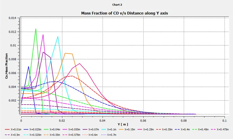
The chart for the change in the mass fraction of Carbon Dioxide along the Y-axis at various lines along X-axis is shown below.
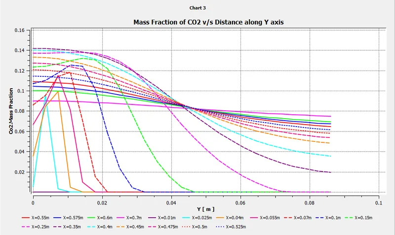
The chart for the change in the mass fraction of the oxides of Nitrogen along the Y-axis at various lines along X-axis is shown below.
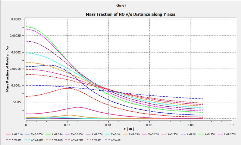
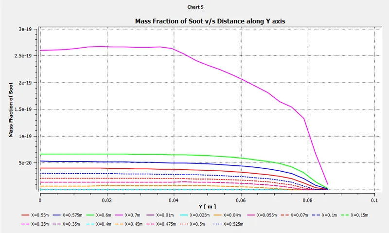
The chart for the change in the Mass fraction of Soot along the Y-axis at various lines along X-axis is shown below.
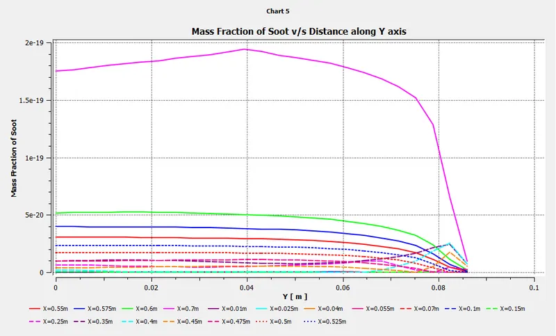
The animation of the Temperature contour can be accessed using the link https://drive.google.com/file/d/1YHLsZVPpE6ZrIadtlyV5R-4VH4ozb5UX/view?usp=sharing
Case 4: 80% CH4 and 20% water(H2O)
Here, 20% of water by mole fraction is added to study the change is results.
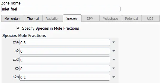
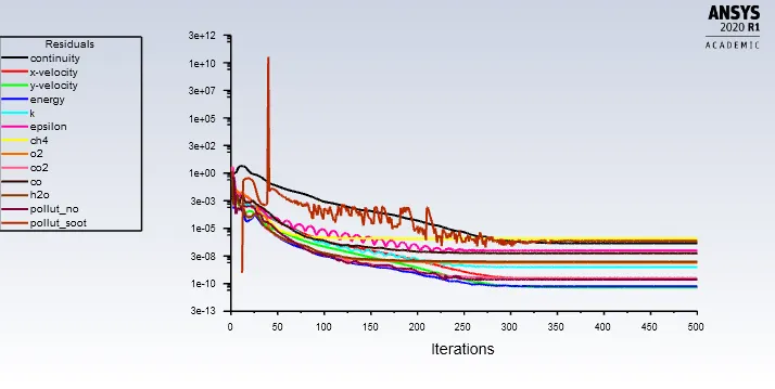
The solution is then run for 500 iterations with the setup mentioned above. The scaled residuals are shown below and it quite evident that the solution is converged.
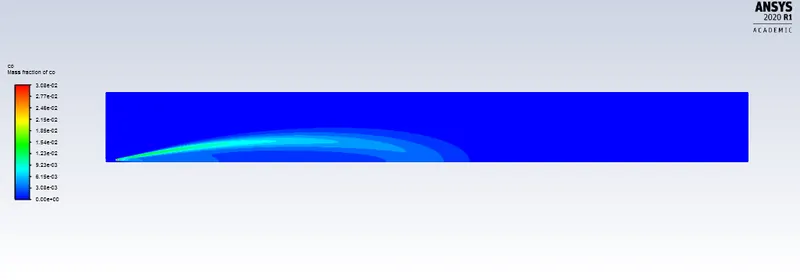
The contour of the mass fraction of CO is shown below.
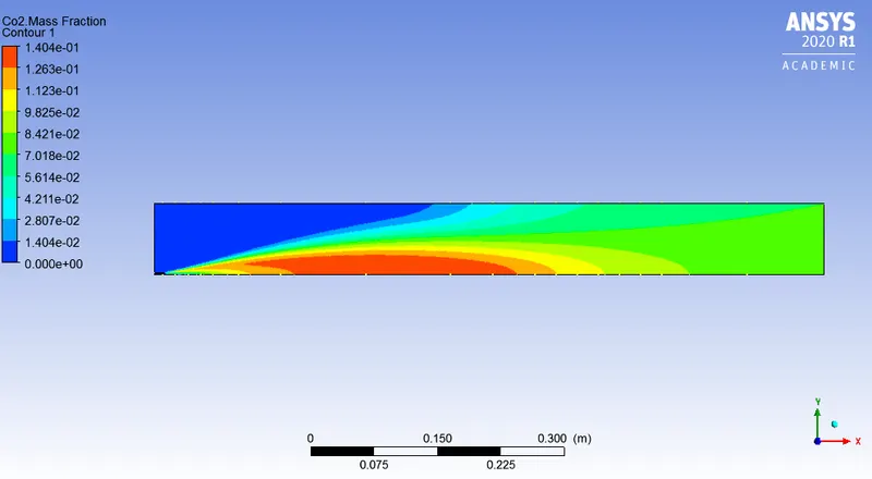
The contour of the mass fraction of CO2 is shown below.
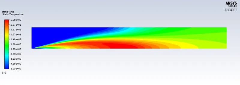
The contour of the temperature is shown below. The peak temperature attained is 2260K.
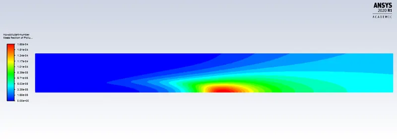
The contour of the mass fraction of the pollutant NO is shown below.
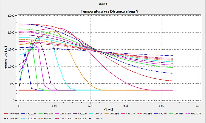
The chart for the change in Temperature along the Y-axis at various lines along X-axis is shown below.
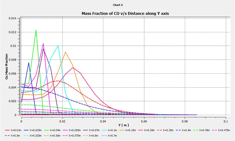
The chart for the change in the mass fraction of Carbon Monoxide along the Y-axis at various lines along X-axis is shown below.
The chart for the change in the mass fraction of Carbon Dioxide along the Y-axis at various lines along X-axis is shown below.
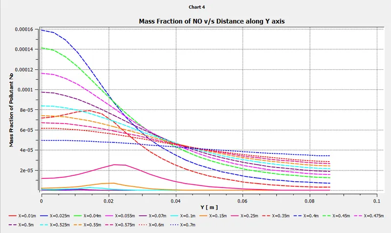
The chart for the change in the mass fraction of the oxides of Nitrogen along the Y-axis at various lines along X-axis is shown below.
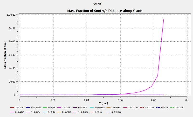
The chart for the change in the mass fraction of Soot along the Y-axis at various lines along X-axis is shown below.
The animation of the Temperature contour can be accessed using the link https://drive.google.com/file/d/1MrCE61GA9Y5n1_Ybcqw2BfHxj2uk6qzo/view?usp=sharing
Case 5: 70% CH4 and 30% water(H2O)
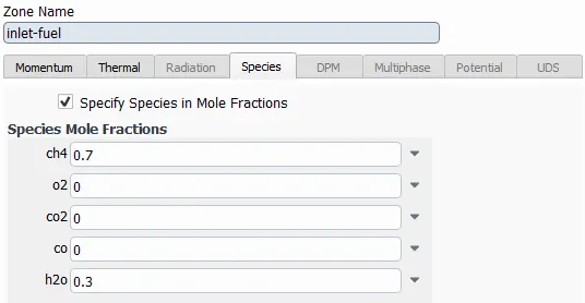
Here, 30% of water by mole fraction is added to study the change is results.
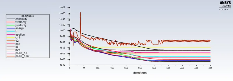
The solution is then run for 500 iterations with the setup mentioned above. The scaled residuals is shown below and it quite evident that the soution is converged.
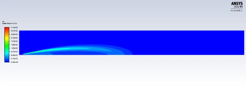
The contour of the mass fraction of CO is shown below.
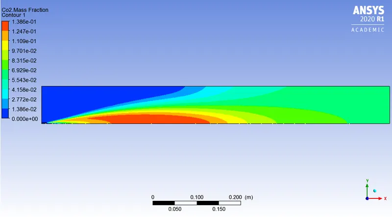
The contour of the mass fraction of CO2 is shown below.
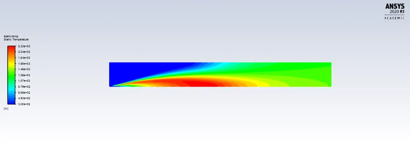
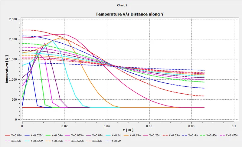
The contour of the temperature is shown below. The peak temperature attained is 2230K.
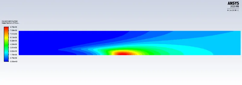
The contour of the mass fraction of the pollutant NO is shown below.
The chart for the change in Temperature along the Y-axis at various lines along X-axis is shown below.
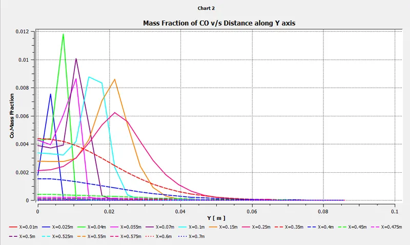
The chart for the change in the mass fraction of Carbon Monoxide along the Y-axis at various lines along X-axis is shown below.
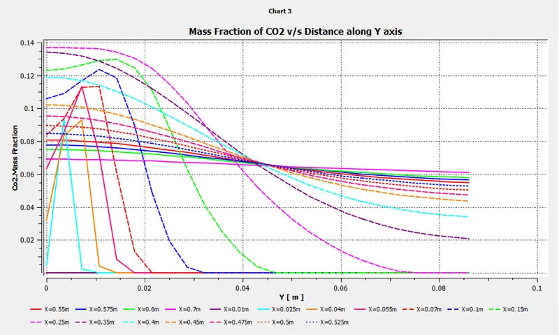
The chart for the change in the mass fraction of Carbon Dioxide along the Y-axis at various lines along X-axis is shown below.
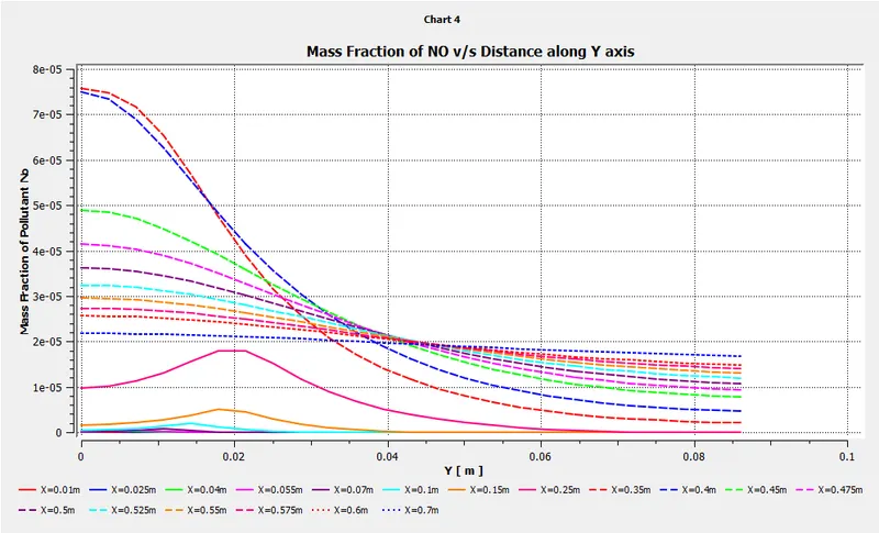
The chart for the change in the mass fraction of the oxides of Nitrogen along the Y-axis at various lines along X-axis is shown below.
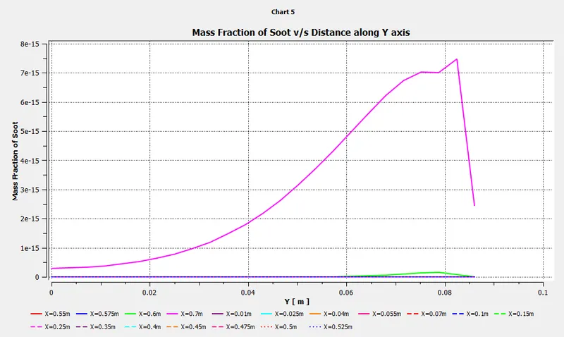
The chart for the change in the Mass fraction of Soot along the Y-axis at various lines along X-axis is shown below.
The animation of the Temperature contour can be accessed using the link https://drive.google.com/file/d/1MCxYLTTO4689nswFvluecaIBNL2cZOSa/view?usp=sharing
Parametric Comparison
| Trial Number | Mole fraction of Methane (CH4) | Mole fraction of Water (H2O) | Peak Temperature in K | Highest concentration of Mass fraction of Carbon Monoxide(CO) | Highest concentration of Mass fraction of Carbon Dioxide(CO2) | Highest concentration of Mass fraction of Oxides of Nitrogen(NOx) | Highest concentration of Mass fraction of Soot |
| Case 1 | 1 | 0 | 2.31e3 | 1.345e-2 | 1.429e-1 | 4.25e-4 | 3.225e-11 |
| Case 2 | 0.95 | 0.05 | 2.30e3 | 1.42e-2 | 1.423e-1 | 3.48e-4 | 1.88e-11 |
| Case 3 | 0.9 | 0.1 | 2.29e3 | 2.40e-2 | 1.417e-1 | 2.80e-4 | 1.08e-11 |
| Case 4 | 0.8 | 0.2 | 2.26e3 | 3.08e-2 | 1.404e-1 | 1.68e-4 | 4.04e-12 |
| Case 5 | 0.7 | 0.3 | 2.23e3 | 3.12e-2 | 1.386e-1 | 8.76e-5 | 1.38e-12 |
Conclusion
- All the trials conducted were mainly to monitor the change in the levels of major pollutants such as Carbon Dioxide(CO2), Oxides of Nitrogen(NOx) and Soot.
- From the above table, it is quite evident that as the percentage of water in the fuel increased, the level of all the pollutants decreased. Hence, there is clearly an inverse proportionality.
- Not only the pollutants, but also there was a drop in the peak temperature as the water in the fuel increased. But, the addition of water can adversely affect the performance of the combustor. Hence, it has to be considered.
- There seems to be an increase in the Carbon Monoxide(CO) levels with increasing level of water in the reaction. This is not a good development as CO is tasteless, odorless and toxic for human beings and animals with haemoglobin.
- However, this challenge simply gives an overview of how the simulation has to be done. In an engineering simulation, the number of species and the reactions will be far more compared to this simulation. Also, the simulation was carried out on a simple combustor and hence we could use the axisymmetric approach. This may not be feasible in real-world simulations.