code that can solve an Otto cycle and make plots for it.

AIM: Write code that can solve an Otto cycle and make plots for it.

Theory

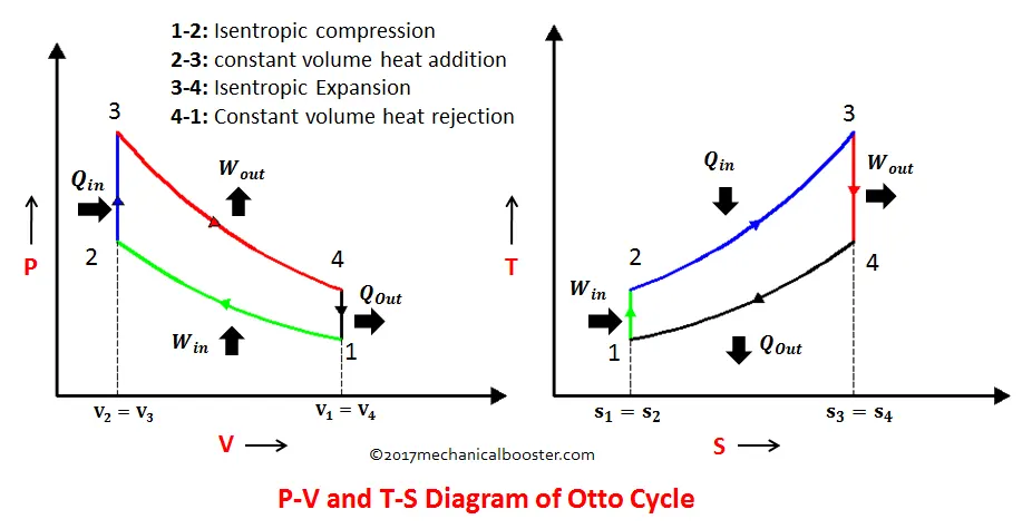
Otto cycle is an ideal thermodynamic combustion cycle, as follows: a compression at constant entropy; a constant-volume heat transfer to the system; an expansion at constant entropy; and a constant-volume heat transfer from the system. The thermal efficiency of the ideal Otto cycle increases with an increasing compression ratio. An actual version of this cycle used in internal combustion engines.

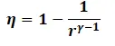
The thermal efficiency of the Otto cycle is:

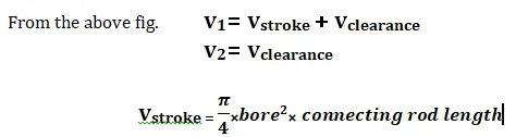
The pressure volume relation during isentropic process in term of engine parameter is:

Where, v= Actual Volume

V_c= clearance volume

r = compression ratio

R = connecting rod length / crank radius

Θ = crank angle

Crank radius = stroke length /2

Ideal gas equation : PV = nRT

Code synopsis

Let us assume the following input for the piston kinematics

Bore = 0.1 m

Stroke length = 0.1 m

Connecting rod length = 0.15 m

Inlet air temp. = 500 K

Inlet air pressure = 1 Bar = 101325 N/m²

Maximum air temp in the cycle = 2300 K

Compression ratio (r) = 12

Process 1-2, is an isentropic compression so apply P₁V₁ = P₂V₂ to get the value for temperature of air after compression i.e. T₂.

Process 2-3 is constant volume heat addition, since air is an ideal gas thus we the ideal gas equation; , to get the value P₃.

Process 3-4, is an isentropic expansion so apply P₃V₃ = P₄V₄ to get the value for temperature of air after compression i.e. T₄.

Code:

close all
clear all
clc
% calculation of otto cycle

%state inputs 
%inlet pressure (N/m2)
p1 = 101325 

% inlet temp. (K)
t1 = 500
t3 = 2300 

%polytopic index of air 
 gamma = 1.4
 
 %compression ratio (dimensionless)
 r=12
 
 %geometry parameter (all dimension in meter)
 bore = 0.1
 stroke = 0.1
 con_rod = 0.15
 
 %calculation of swept volume and clearance volume
 v_swept = (pi/4)*bore^2*stroke
 
 %r= (v_clear+v_swept/v_clear)
 v_clear= v_swept/(r-1)
 
v1 = v_clear + v_swept
v2 = v_clear
 
%state variable at state 2
%p1*v1^gamma = p2*v2^gamma
p2= p1*(v1/v2)^gamma

%t1*v1^(gamma-1) = t2*v2^(gamma-1)
t2 = t1*(v1/v2)^(gamma-1)

constant_c = p2*v2^gamma;
v_compression= piston_kinematics(bore,stroke,con_rod,r,0,180);
P_compression = constant_c./v_compression.^gamma;

constant_c = t2*v2^(gamma-1);
t_compression=constant_c./v_compression.^(gamma-1);

%state variable at state 3
v3=v2
 %use ideal gas equation ((p2/t2)=(p3/t3))
 p3=p2*(t3/t2)
 
 constant_c = p3*v3^gamma;
v_expansion= piston_kinematics(bore,stroke,con_rod,r,180,0);
P_expansion = constant_c./v_expansion.^gamma;

constant_c = t3*v3^(gamma-1);
t_expansion=constant_c./v_expansion.^(gamma-1);
 
%state variable at state 4
v4 =  v1
%p3*v3^gamma = p4*v4^gamma
p4= p3*(v3/v4)^gamma

%t3*v3^(gamma-1) = t4*v4^(gamma-1)
t4 = t3*(v3/v4)^(gamma-1)
figure (1)
 hold on
plot(v1,p1,'*','color','magenta')
plot(v_compression, P_compression)
plot(v2,p2,'*','color','magenta')
plot(v3,p3,'*','color','magenta')
plot(v_expansion, P_expansion)
plot(v4,p4,'*','color','magenta')
plot([v2, v3],[p2, p3],'color','b')
plot([v4, v1],[p4, p1],'color','b')
xlabel('Volume')
ylabel('Pressure')

figure(2)
hold on
plot(v1,t1,'*','color','blue')
plot(v2,t2,'*','color','blue')
plot(v_compression,t_compression)
plot(v3,t3,'*','color','blue')
plot(v_expansion,t_expansion)
plot(v4,t4,'*','color','blue')
plot([v2, v3],[t2, t3],'color','b')
plot([v4, v1],[t4, t1],'color','b')
xlabel('Volume')
ylabel('Temperature')

% Thermal efficency of engine
eff = [1-(1/r)^(gamma-1)]*100

Calling Functions are:

% DECLARATION OF PISTON KINEMATICS FUNCTION
function [v]= piston_kinematics(bore,stroke,con_rod,r,start_angle,end_angle)
   %piston kinematics
   bore = 0.1
   stroke = 0.1
   con_rod = 0.15
   r = 12
   v_swept= (pi/4)*bore^2*stroke
   v_clear = v_swept/(r-1);
   theta = linspace(start_angle,end_angle,180);
   cra_radius = stroke/2
   R= con_rod/cra_radius
   %(v/v_clear)= 1+0.5*(r-1)*(R+1-cosd(theta)-(R^2-sind(theta)^2)^0.5)
    A= 0.5*(r-1);
    B= R+1-cosd(theta);
    C= (R^2-sind(theta).^2).^0.5;
    v = (1+A*(B-C))*v_clear; 
end

Output:

p1 =

      101325


t1 =

   500


t3 =

        2300


gamma =

    1.4000


r =

    12


bore =

    0.1000


stroke =

    0.1000


con_rod =

    0.1500


v_swept =

   7.8540e-04


v_clear =

   7.1400e-05


v1 =

   8.5680e-04


v2 =

   7.1400e-05


p2 =

   3.2853e+06


t2 =

   1.3510e+03


bore =

    0.1000


stroke =

    0.1000


con_rod =

    0.1500


r =

    12


v_swept =

   7.8540e-04


cra_radius =

    0.0500


R =

    3.0000


v3 =

   7.1400e-05


p3 =

   5.5931e+06


bore =

    0.1000


stroke =

    0.1000


con_rod =

    0.1500


r =

    12


v_swept =

   7.8540e-04


cra_radius =

    0.0500


R =

    3.0000


v4 =

   8.5680e-04


p4 =

   1.7251e+05


t4 =

  851.2465


eff =

   62.9893

Plots:

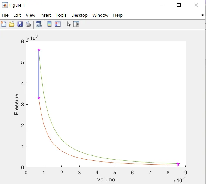
P-V Curve

T-V Curve

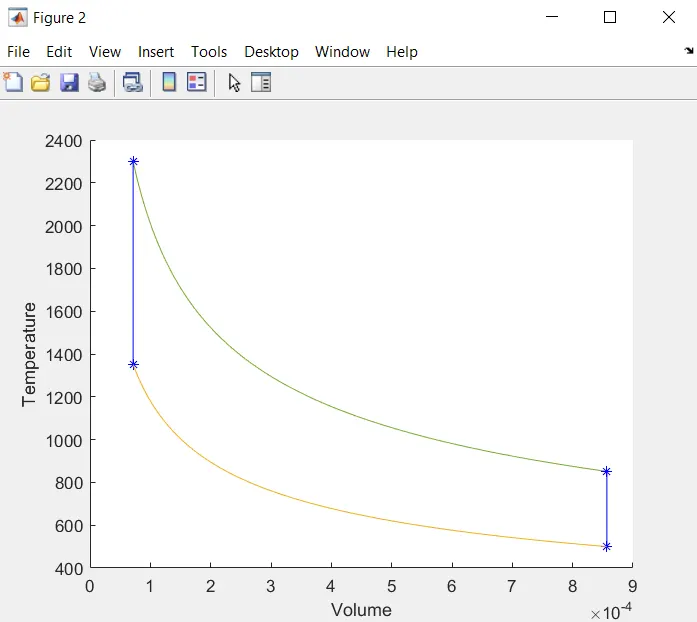
Conclusion:

From the graph it is clearly that curve were smooth and follow the ideal otto cycle and thermal efficiency is 62.938% which is in the range of 56% to 63%.