Channel Flow
AIM
The aim is to simulate the flow inside a rectangular channel
OBJECTIVES
- Simulation has to be run for 3 different cases varying the mesh
- Contour plots of parameters
- Comaparision of results in paraview and Converge post
PIPE FLOW
Pipe flow, a branch of hydraulics and fluid mechanics, is a type of liquid flow within a closed conduit (conduit in the sense of a means of containment). The other type of flow within a conduit is open channel flow. These two types of flow are similar in many ways, but differ in one important aspect. Pipe flow does not have a free surface which is found in open-channel flow. Pipe flow, being confined within closed conduit, does not exert direct atmospheric pressure, but does exert hydraulic pressure on the conduit.
The behaviour of pipe flow is governed mainly by the effects of viscosity and gravity relative to the inertial forces of the flow. Depending on the effect of viscosity relative to inertia, as represented by the Reynolds number, the flow can be either laminar or turbulent. At a Reynolds number below the critical value of approximately 2040[1] pipe flow will ultimately be laminar, whereas above the critical value turbulent flow can persist. In addition, the transition between laminar flow and turbulence can be sensitive to disturbance levels and imperfections.
Flow through pipes can roughly be divided into two:
- Laminar flow
- Turbulent flow
RECTANGULAR CHANNEL FLOW SIMULATION CASE 1
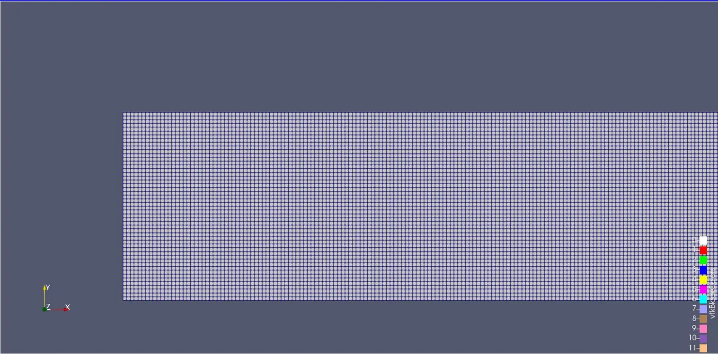
Now there are different mesh setup as shown below
Mesh(2e-4m)
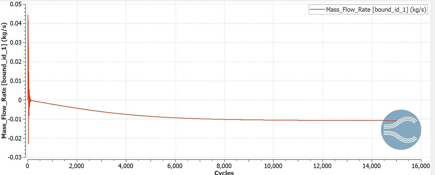
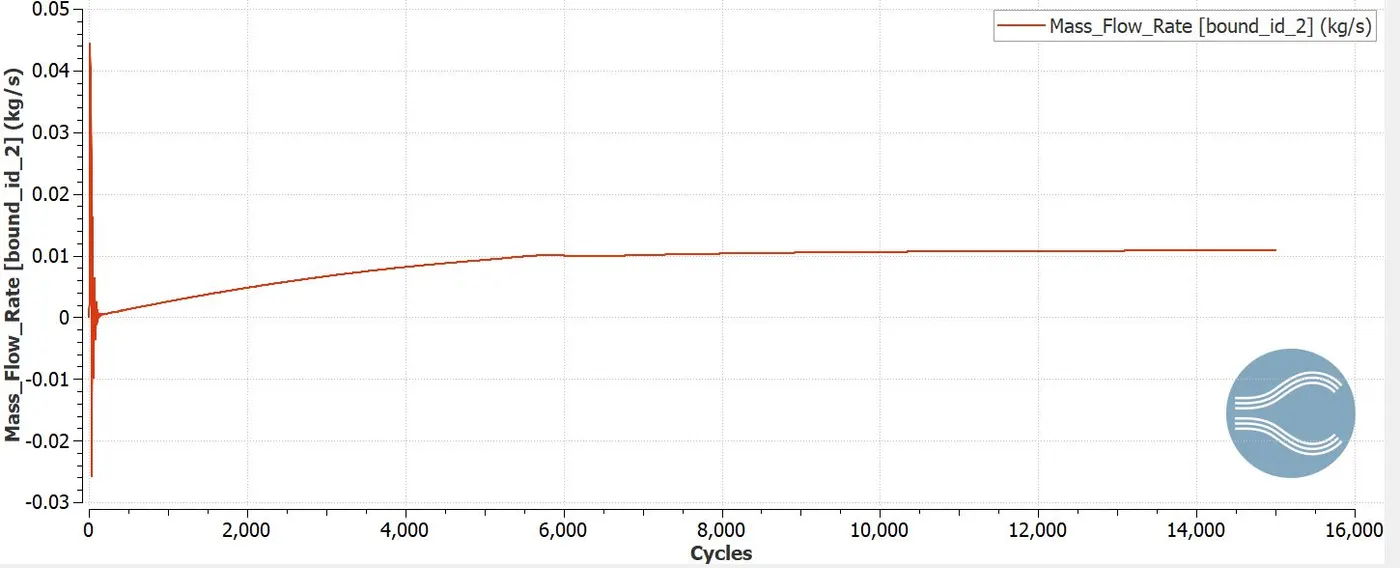
Mass flow rate versus cycles
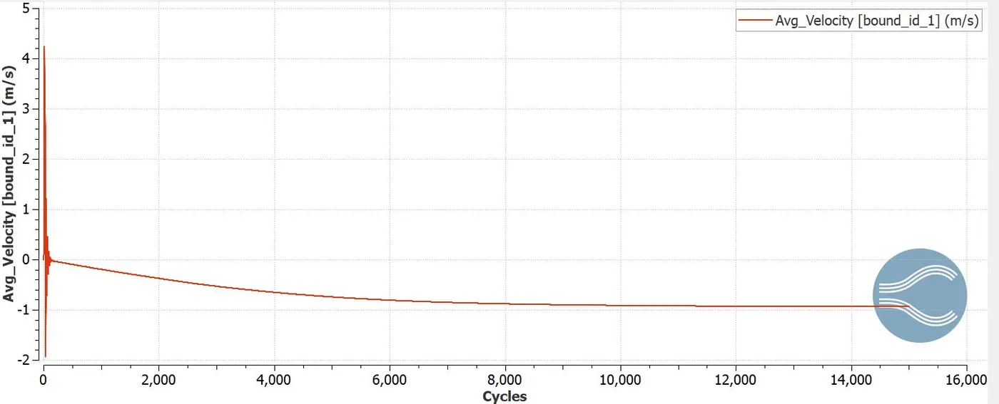
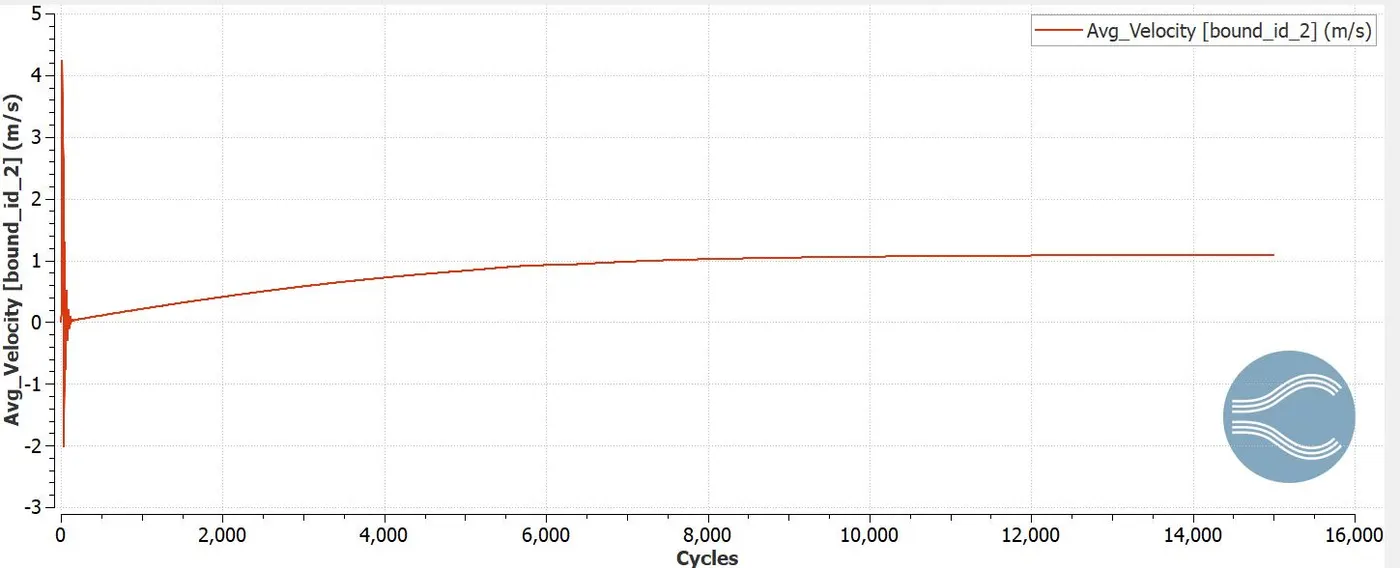
Velocity Versus Cycles
Pressure Versus Cycle
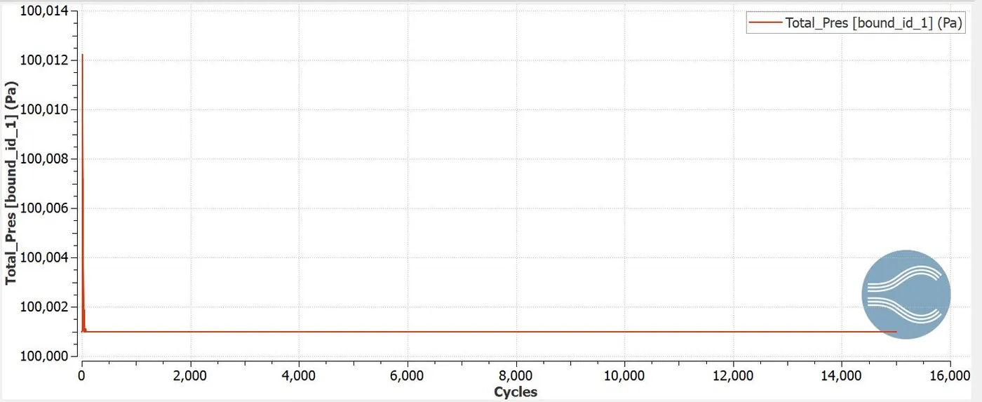
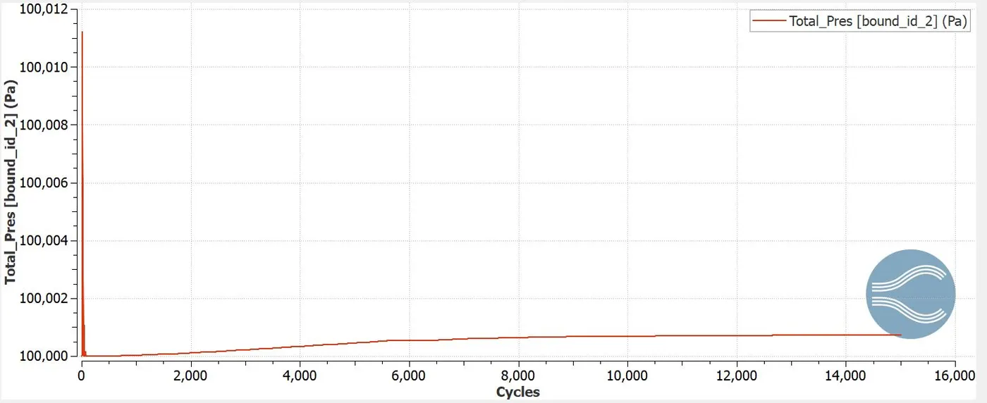
From the above graphs, we observe that there are oscillations at the beginning of the cycle, but as the solution marches ahead in terms of number of cycles the oscillations starts to fade away. This behaviour of the parameters with respect to cycles is known as convergence. The convergence criteria is always defined during setup of the simulation, where the tolerance would be set for error. The solution is marched in time until the tolerance value is less than error. In the above plots there are two graphs one for the inlet and other for the outlet. In the inlet there is positive sign cause the flow is along the normal of the inlet boundary whereas the outlet has converged to negative value as the flow is opposite to the flow direction. This is to ensure the mass, momentum and energy is conserved.
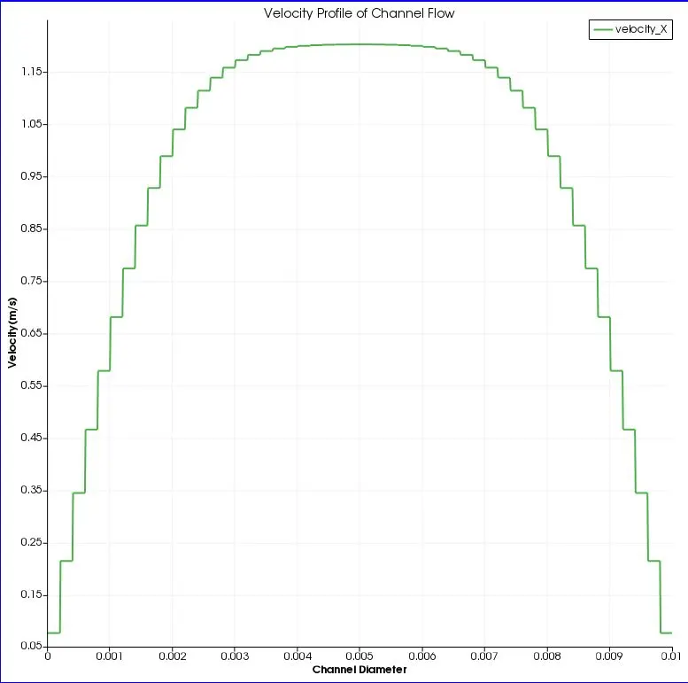
Velocity profile
Pressure Profile
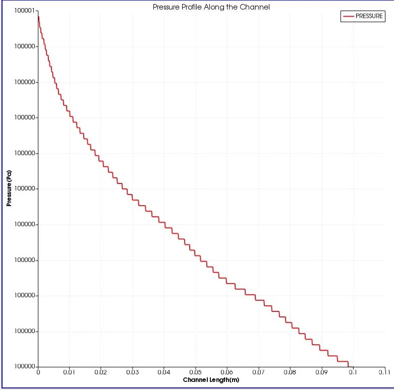
These profiles are in velocity and pressure profiles along and across the channel. As usual the velocity has a parabolic variation, the velocity near the walls is zero but as we reach the axis of the channel the flow velocity is on the maximum value. The pressure plots also sees a non linear variation of pressure along the channel diameter.
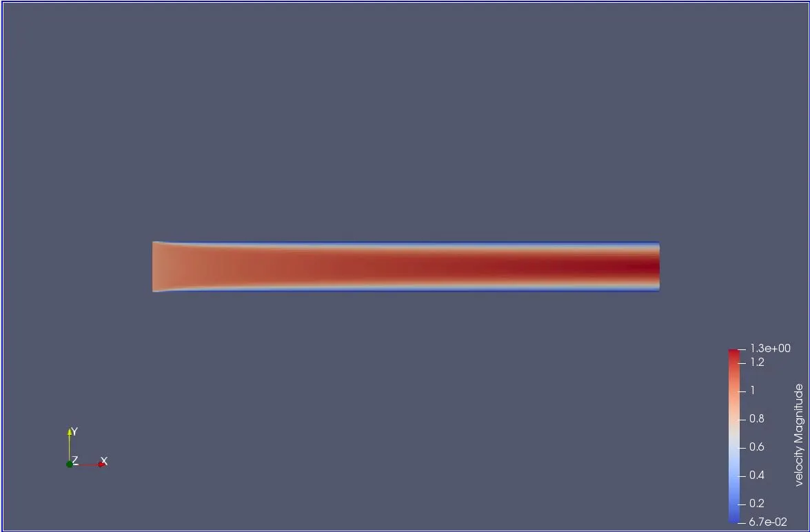
Velocity Contour
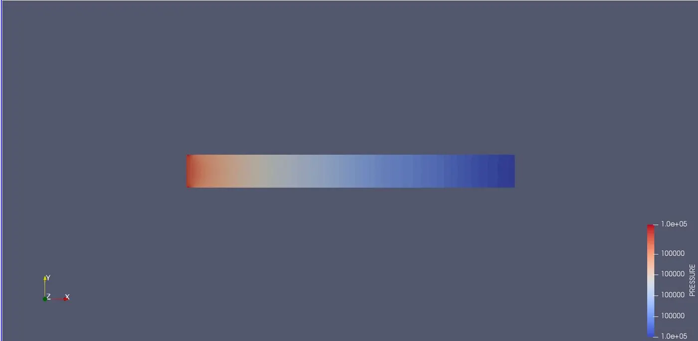
Pressure Contour
RECTANGULAR CHANNEL FLOW SIMULATION CASE 2
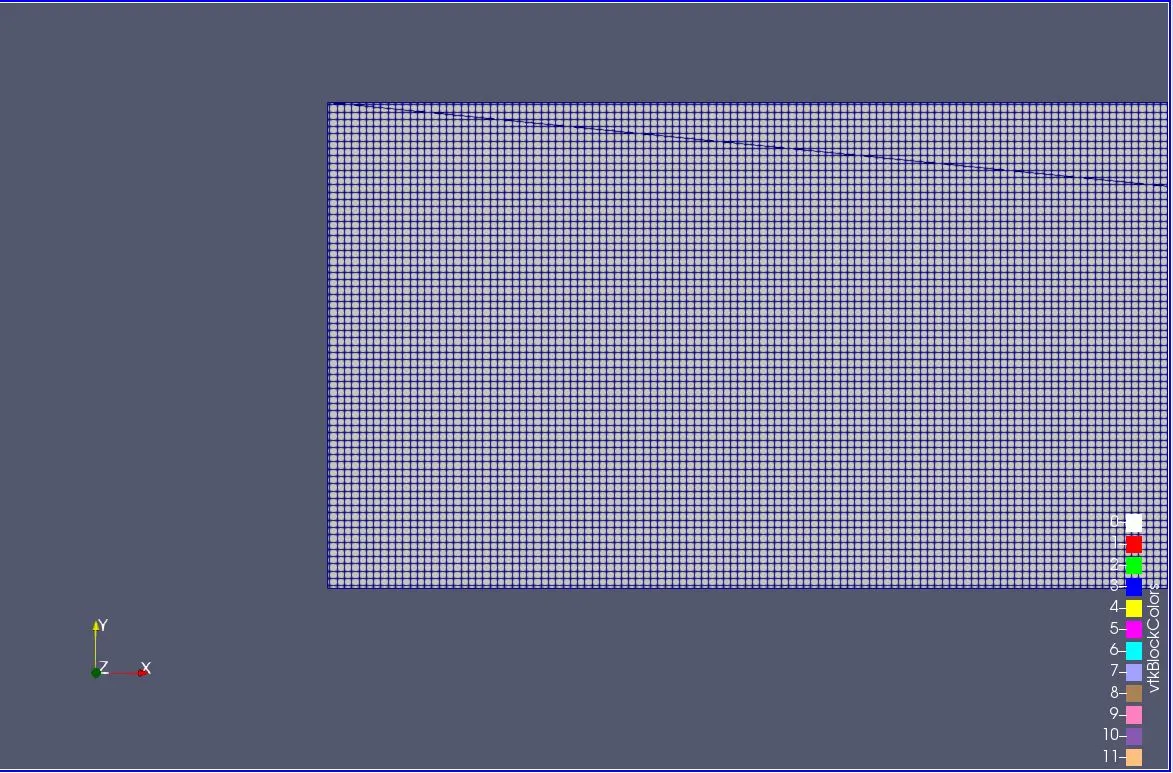
Now there are different mesh setup as shown below
Mesh(1.5e-4m)
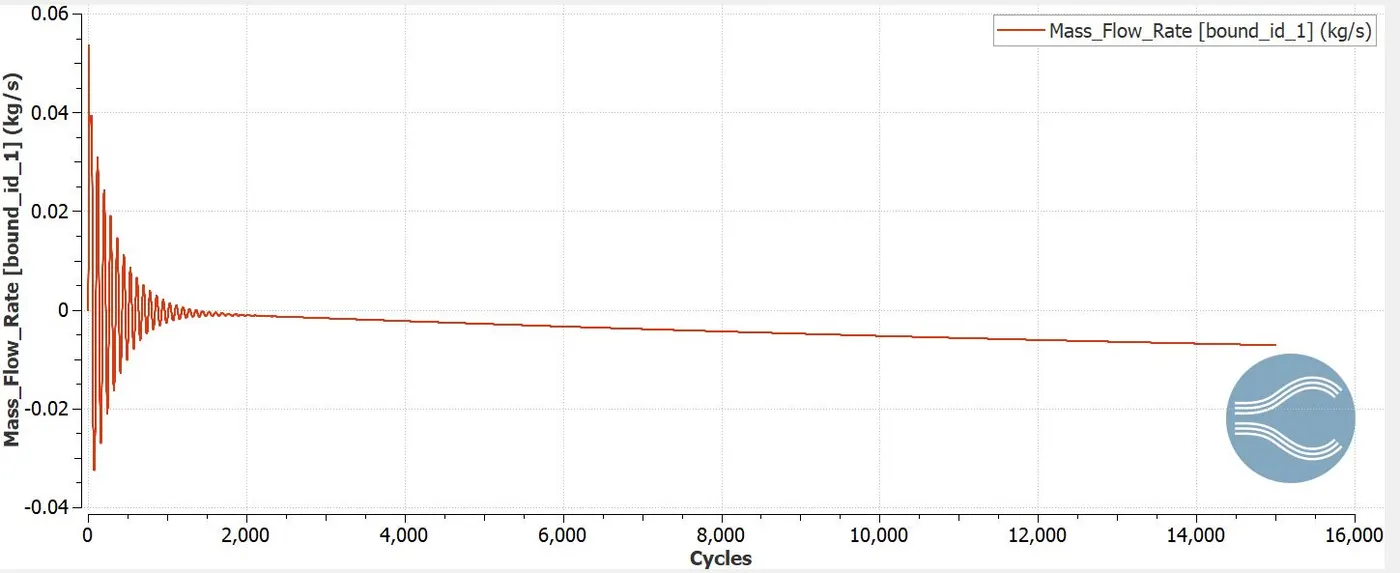
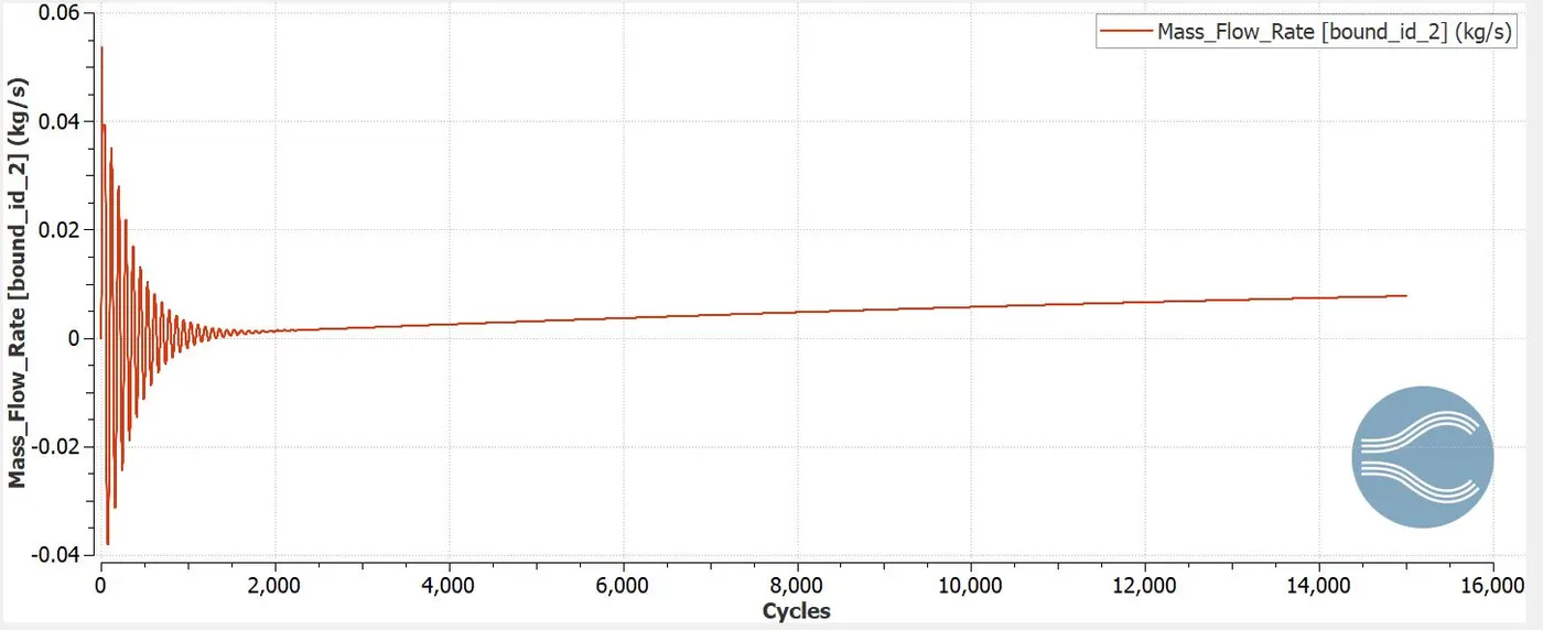
Mass flow rate versus cycles
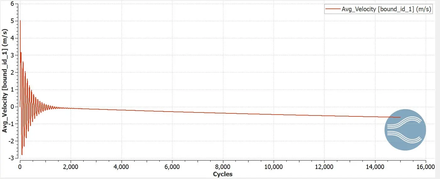
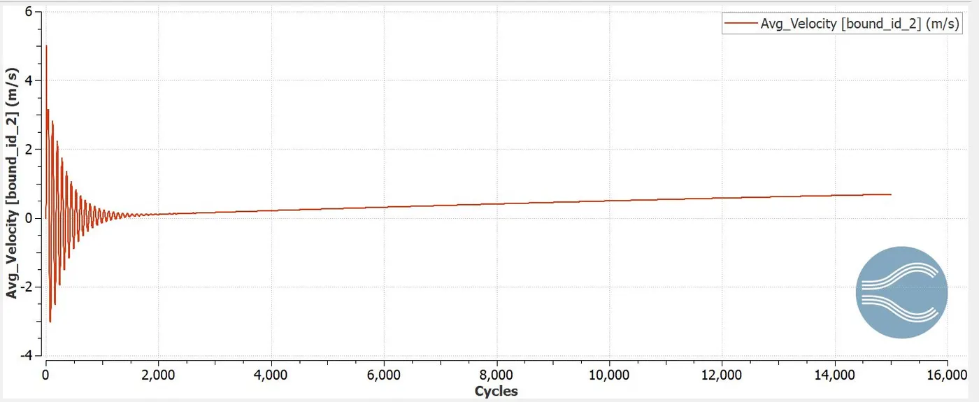
Velocity Versus Cycles
Pressure Versus Cycle
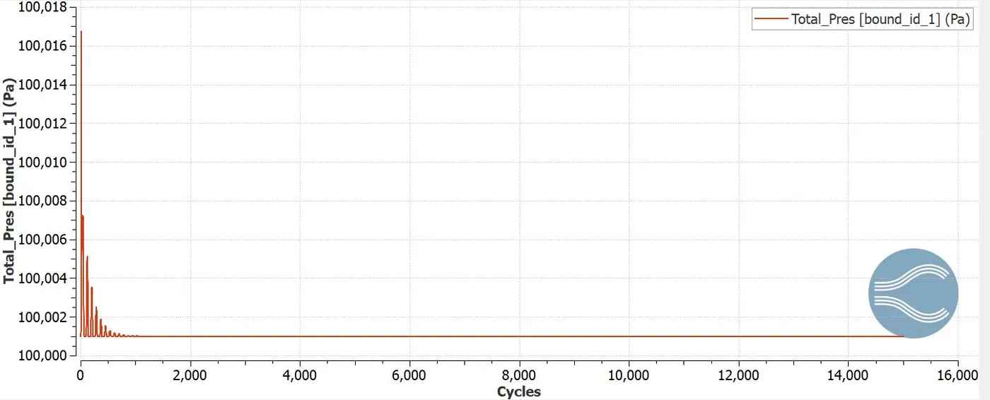
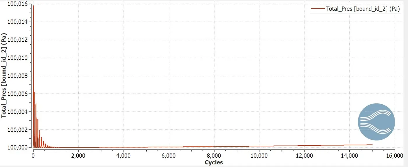
From the above graphs, we observe that there are oscillations at the beginning of the cycle, but as the solution marches ahead in terms of number of cycles the oscillations starts to fade away. This behaviour of the parameters with respect to cycles is known as convergence. The convergence criteria is always defined during setup of the simulation, where the tolerance would be set for error. The solution is marched in time until the tolerance value is less than error. In the above plots there are two graphs one for the inlet and other for the outlet. In the inlet there is positive sign cause the flow is along the normal of the inlet boundary whereas the outlet has converged to negative value as the flow is opposite to the flow direction. This is to ensure the mass, momentum and energy is conserved.
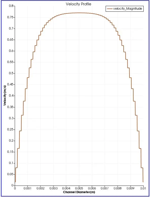
Velocity profile
Pressure profile
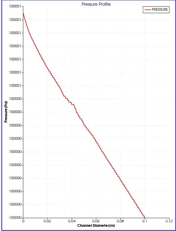
These profiles are in velocity and pressure profiles along and across the channel. As usual the velocity has a parabolic variation, the velocity near the walls is zero but as we reach the axis of the channel the flow velocity is on the maximum value. The pressure plots also sees a non linear variation of pressure along the channel diameter.
Velocity Contour
Pressure Contour
RECTANGULAR CHANNEL FLOW SIMULATION CASE 3
Now there are different mesh setup as shown below
Mesh(1.2e-4m)
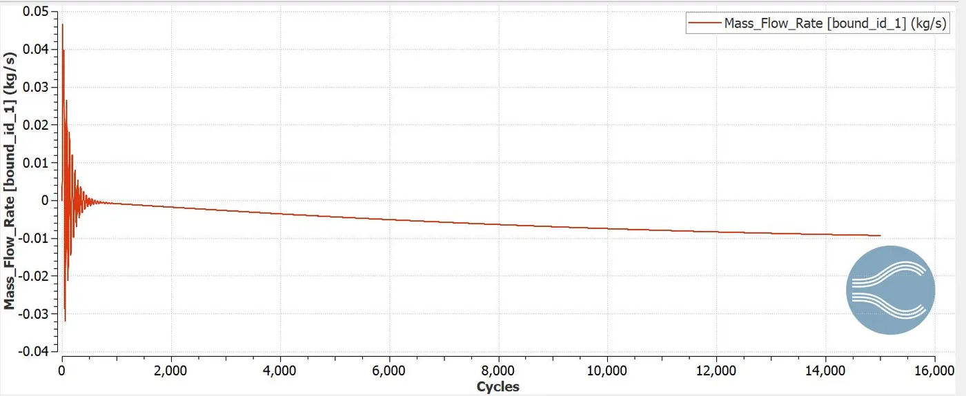
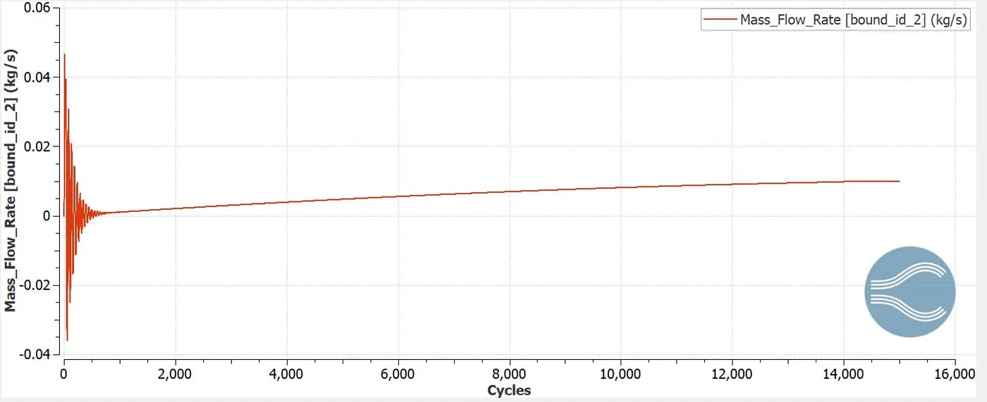
Mass flow rate versus cycles
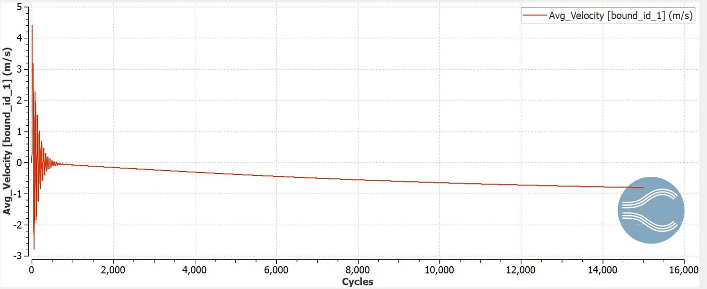
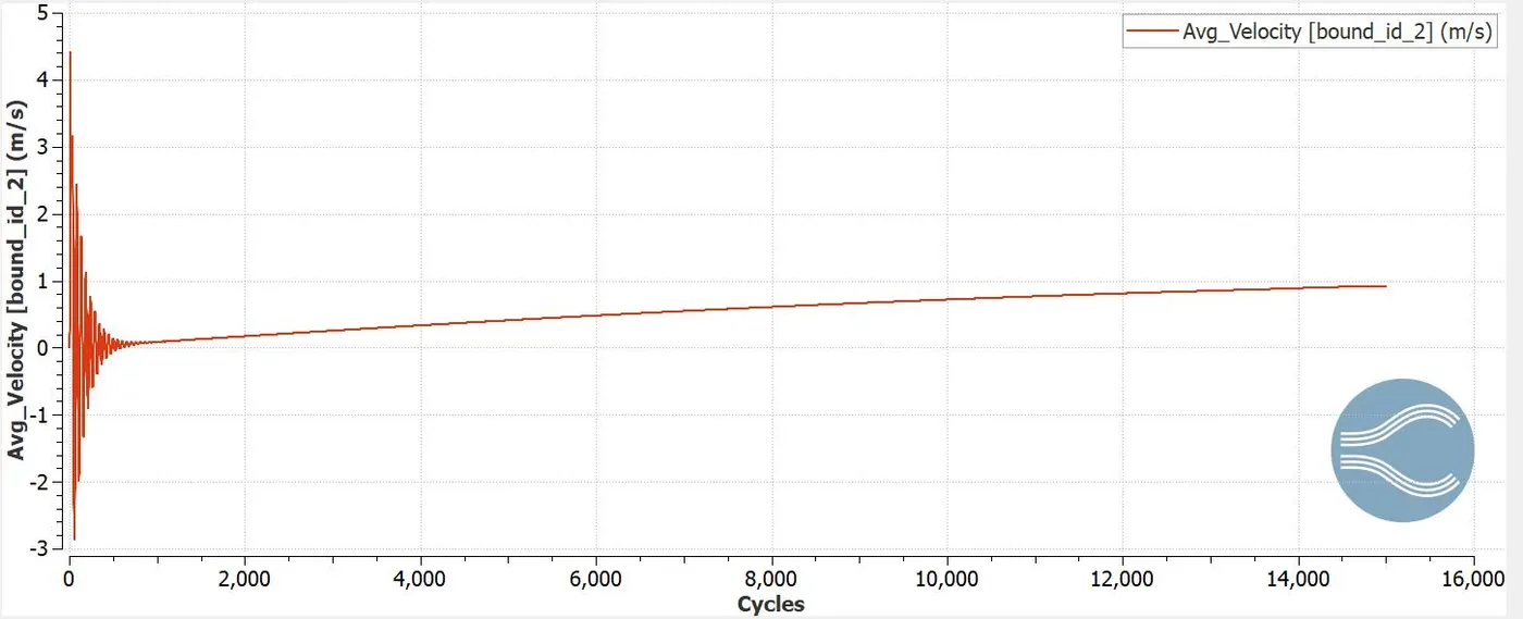
Velocity Versus Cycles
Pressure Versus Cycle
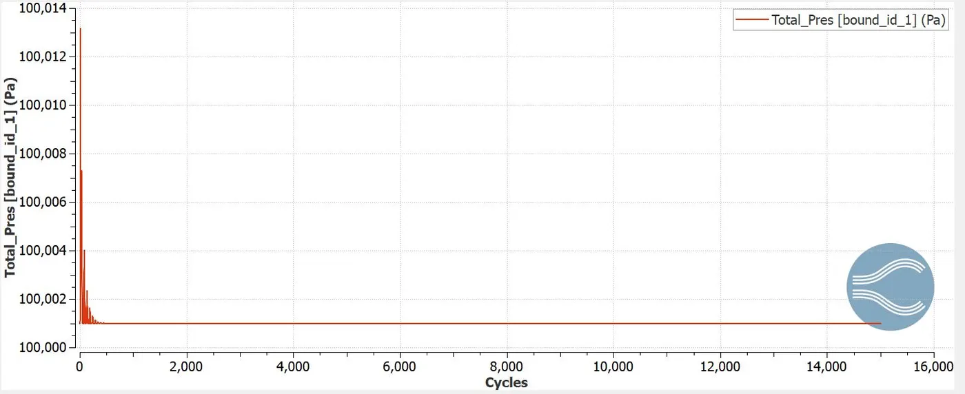
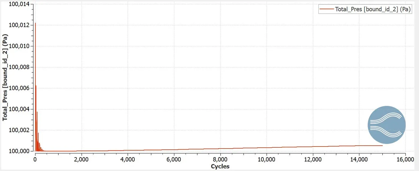
From the above graphs, we observe that there are oscillations at the beginning of the cycle, but as the solution marches ahead in terms of number of cycles the oscillations starts to fade away. This behaviour of the parameters with respect to cycles is known as convergence. The convergence criteria is always defined during setup of the simulation, where the tolerance would be set for error. The solution is marched in time until the tolerance value is less than error. In the above plots there are two graphs one for the inlet and other for the outlet. In the inlet there is positive sign cause the flow is along the normal of the inlet boundary whereas the outlet has converged to negative value as the flow is opposite to the flow direction. This is to ensure the mass, momentum and energy is conserved.
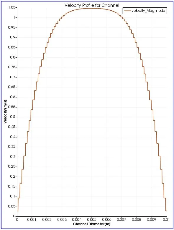
Velocity profile
Pressure Profile
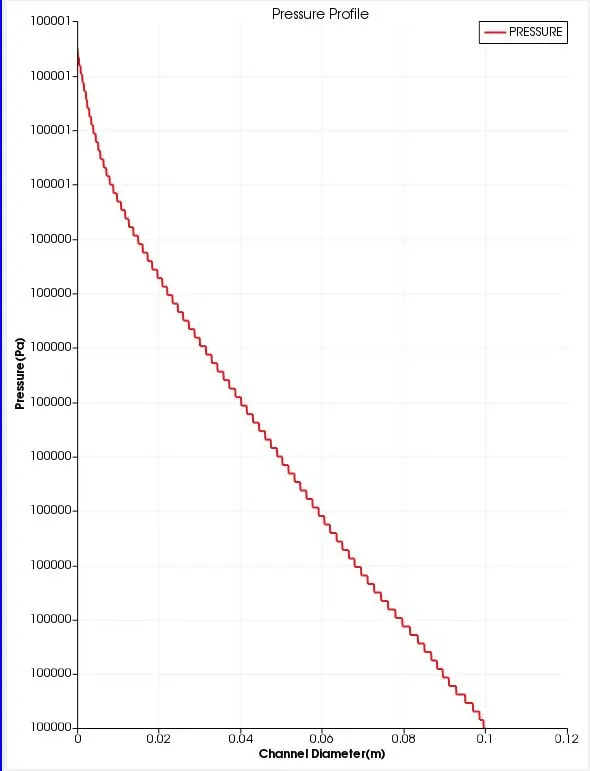
These profiles are in velocity and pressure profiles along and across the channel. As usual the velocity has a parabolic variation, the velocity near the walls is zero but as we reach the axis of the channel the flow velocity is on the maximum value. The pressure plots also sees a non linear variation of pressure along the channel diameter.
Velocity Contour
Pressure Contour
ANIMATIONS FOR VELOCITY AND PRESSURE
CONCLUSION
- The flow inside the channel was simulated
- The various plots were analysed for flow variables
- Flow parameters were plotted
- The velocity and pressure animations shows the behaviour of the fluid in the channel