Bird Strike - Project - 2

Simulation of Bird Strike Using LS-Dyna

1. Introduction

A bird strike is strictly defined as a collision between a bird and an aircraft that is in flight or on a takeoff or landing roll.

Bird Strike is common and can be a significant threat to aircraft safety. For smaller aircraft, significant damage may be caused to the aircraft structure and all aircraft, especially jet-engined ones, are vulnerable to the loss of thrust which can follow the ingestion of birds into engine air intakes. This has resulted in a number of fatal accidents.

Bird strikes may occur during any phase of flight but are most likely during the take-off, initial climb, approach and landing phases due to the greater numbers of birds in flight at lower levels. Since most birds fly mainly during the day, most bird strikes occur in the daytime. Most fatal are the ones in which bird gets ingested into the engines and damage the rotors and cause explosions.

Fig 1.1: the damage caused to the aircraft engine rotors due to a bird strike

Problem statement:

This is a classic nonlinear transient dynamics problem similar to car crashes and mobile drops. While accurate modelling of the problem requires advanced techniques such as SPH (Smooth Particle Hydrodynamics), this problem can be solved using a generic explicit solver. Here is the information required to model the phenomenon.

• The blades should rotate at a constant velocity but the casing should remain stationary.
• The cylindrical bird model should travel along its own axis and hit the blades.
• Use elastic material for the bird (2000MPa) and the casing (200GPa). The material model for the blades is attached.
• The velocity of the engine blades and the birds can be chosen so that blade failure can be seen within a short span of time.

Apart from this, meshed file of the model was provided and it was asked to keep all the parts, keywords like contacts, boundary conditions, material data and control files into separate key files and unite them together in the main file.

2. The geometry

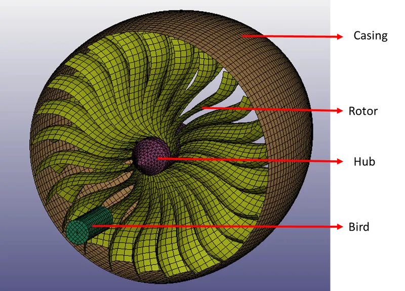
Fig 2.1: The geometry provided for the exercise

All these pars were put into separate files and section properties were assigned to them. All the parts except the hub were meshed with shell mesh. The hub was meshed using the tetra elements. A renumbering according to below given scheme was done for all the parts:

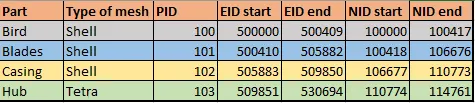
Table: Renumbering scheme followed for the model

Such renumberings enable different teams to work simultaneously on subsystems of a large model. Element formulation 2 was used for all the shell elements and 10 was used for the hub which was meshed with tetra elements.

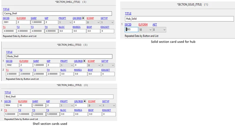
Fig 2.2: The section cards used for various parts

Note the bird was made stiffer by assigning more thickness as we were not much interested in the impact on the bird. While assigning the element formulations the, compatibility of different element formulations with different element types was kept in mind. For the tetra elements, element formulations 4 or 10 need to be used. Each section card was assigned to the parts in their respective part files.

3. Material cards

A material card for the rotor blade was provided as a part of the exercise. It was a MAT_024_piecewise linear plasticity model as shown in the below-attached figure.

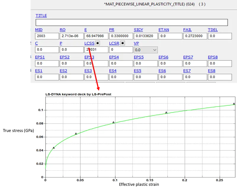
Fig 3.1: The piecewise linear plasticity model used for blades

Further 3 more materials were modelled for bird, casing and the hub. An elastic material card was used for the bird material while piecewise linear plasticity cards were used for the casing and the hub as shown in the below-attached figure. The material properties were similar to steel for the casing, hard rubber for the bird and high strength alloy for the hub.

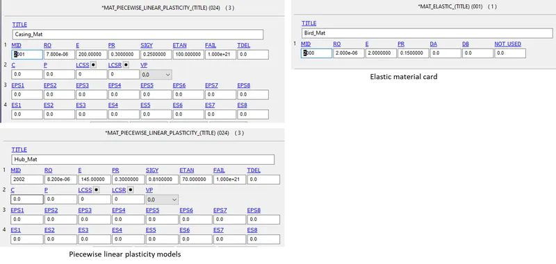
Fig 3.2: The material models used for casing, hub and the bird

4. Boundary Conditions

The casing was fixed using SPC (single point constraint) with all the DOFs constrained. The rotor blades was provided a rotation at 0.5 rad/ms which translates to 5000 rpm. This was achieved by using a velocity generation card available in the initial keyword. Then the bird model was assigned a linear velocity of 20mm/ms which translates to 72 kmph. This was again achieved using the velocity generation card.

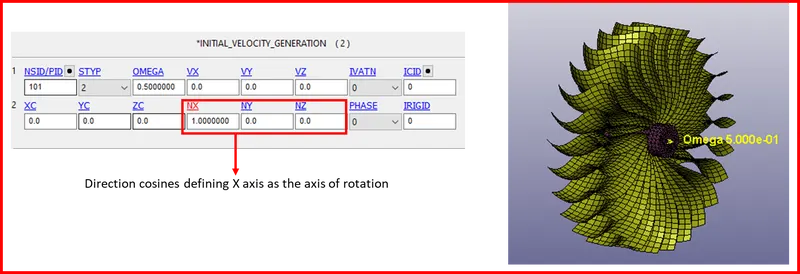
Fig 4.1: The rotation applied to the rotor blades

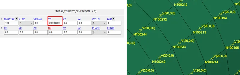
Fig 4.2: The linear velocity applied to bird model using velocity generation card

5. Contacts

Contacts are vital parts of FE modelling, they define the interaction between different elements and enable the solver to avoid penetration of elements from one part into another. In this exercise, three types of contacts were used. The first one is automatic surface to surface contact defined between bird-rotor and rotor-casing. The second contact card used is tied nodes to surface contact, it is basically used to define a rigid joint between two parts. This card was used for rotor blades and hubs making them move together. The third card was automatic single surface contact. It was used to avoid rotor blades from self penetration during deformation.

It is good practice to avoid repeating of same contact card so, for the automatic surface to surface contact modelling, the master entities were put as the part set containing the bird and casing. The slave part was put as a part - the rotor blade. It was done as we expect the deformation to happen on the rotor blades. Note: we intentionally increased the stiffness of the bird part as we did not want an elaborate study of damage to it.

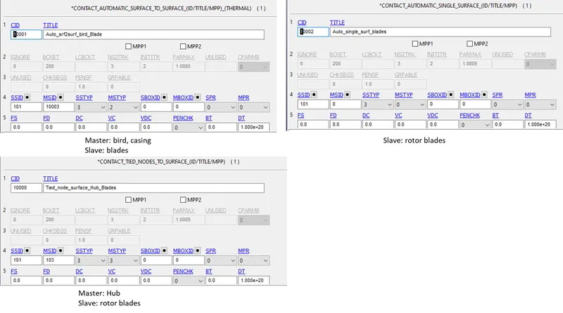
Fig 5.1: The contact cards used for the model

6. Control cards

The nature of the problem is dynamic transient and nonlinear so the explicit scheme is used for solving the model. A termination time of 5 ms was used by using the control termination keyword. Hourglass control was used as blades were subjected to bending and buckling upon impact. The control timestep card was used for the purpose of mass scaling to bring down the solution time for the simulation. The effects on the runtime are discussed in a separate section.

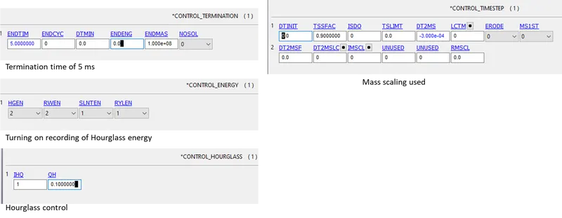
Fig 6.1: The control cards used in the model

7. Database

Output requests are made using the database keyword. ASCII option was used to enable recording of GLSTAT (energies), SLEOUT (sliding energy at contact interface) and Hourglass energy at an interval of 0.01ms. D3PLOT keyword was used for recording the animation and history data.

8. Organising all the files into the main file.

*include keyword is used for calling in separate files into the main file. This comes in handy in the event of a team working on different subsystems of a complex model and later on assembling all of them for running the simulation. The below figure shows all the referenced files which were kept in the same folder. This eliminates the need of complicated mentioning of different directories in the *Include keyword.

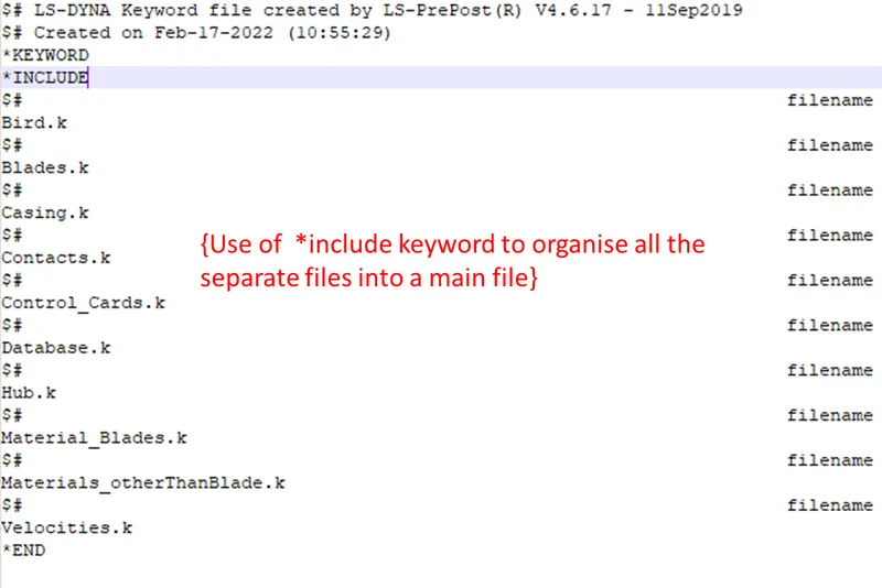
Fig 8.1: The use of *Include keyword for calling all the individual files

9. Mass scaling

After giving the run command for the model, the message window displays the estimated time to complete the simulation. For large models, this time can be pretty large depending on the minimum element length present in the model. Basically, the explicit solver timestep size is calculated based on the minimum element length present in the model. This can be improved using the technique of mass scaling. It can be achieved using the DT2MS value and TSSFAC values in the control timestep card. If a positive value is used in the DT2MS value, the addition of artificial mass to the elements that lead to a reduction in timestep size happens while mass is reduced for those elements where the timestep size increases a certain value. This method is not usually recommended. Another way is to use negative values, in this case only addition happens for smaller sized elements and oversized ones are not disturbed. It is preferred and leads to the addition of artificial mass in the system leading to an increase in Internal energy. This needs to be controlled below 7-8% so that the results are not affected significantly.

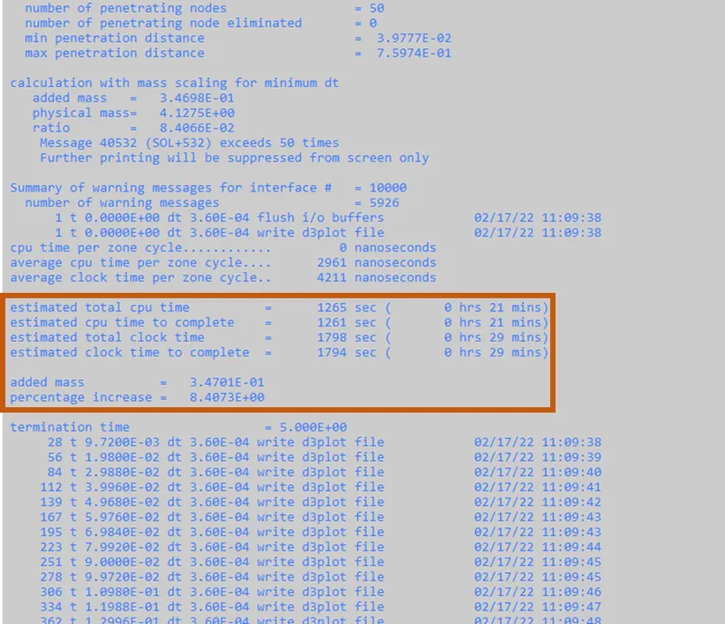
Fig 9.1 The mass scaling brought down the original estimated time of 1 Hr 26 min to 29 mins

Since an increase of 8% mass was there in this setup, a reduced one with almost 2% mass addition at DT2MS= 3e-5 was used.

10. Results and discussion.

Animation: The result of the simulation

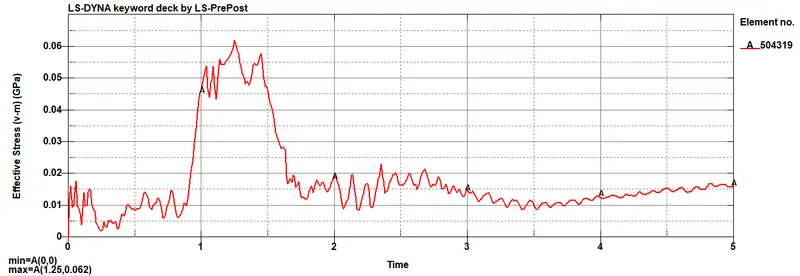
Fig 10.1: The effective stress plot for an element belonging to the blade where contact happens initially

The rise at t=1ms signifies the impact which is followed by relaxation as expected for a material modelled using a piecewise linear plasticity model. The maximum stress was 62 MPa which is above yield stress (13.3 MPa ) but below the failure value of 272 MPa. This leads to deformation but not a detachment of the impacted portion.

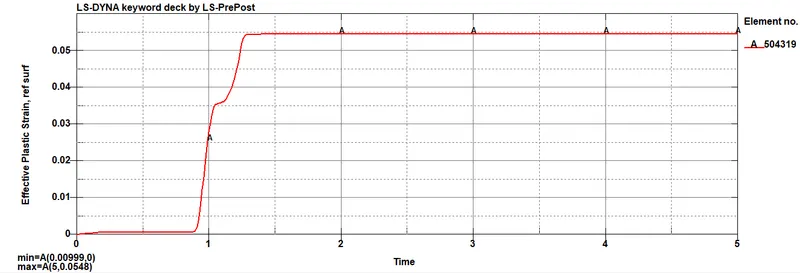
Fig 10.2: The effective plastic strain in the element where the impact happens

Significant deformation of 5% is apparent from the plot which signifies loss of functionality for the rotors.

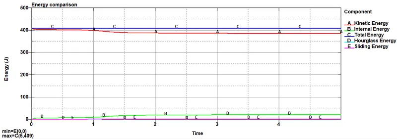
Fig 10.3: The comparison of different system energies

The total energy remains constant and internal and kinetic energy plots are opposite to each other in a manner similar to outcomes of crash tests. Also, the hourglass and sliding energies are negligible, so our simulation was k from this point of view.

11. Conclusion

• The bird strike is a nonlinear, transient and dynamic problem that can be simulated using explicit solvers within very optimised time.
• For complex models, the use of a multi-file system makes it easier for modelling as different teams can work on different subsystems simultaneously.
• The standardised numbering system makes things further easier for the CAE engineers.