Basics of ML & AL Week 2 Challenge

First Business Moment (Measure of Central Tendency)

Mean (`\mu`) =`sum (x_i)* P(x)`= expected value

Therefore, `\mu`= [(0*0.35) + (1*0.25) + (2*0.15) + (3*0.15) + (4*0.10)] = 0 + 0.25 + 0.30 + 0.45 + 0.4 Therefore , `\mu` =1.4.

Second Business Moment

Variance (`\sigma ^2`) = `sum (x_i -\mu_x)^2* P(x)`

Therefore, Variance = [`(0-1.4)^2 * 0.35` + `(1-1.4)^2 * 0.25` + `(2-1.4)^2 * 0.15` + `(3-1.4)^2 * 0.15` + `(4-1.4)^2 * 0.1`] = 0.686 + 0.04 + 0.054 + 0.384 + 0.676 = 1.84

Therefore, `sigma`= 1.36.

Third Business Moment (Skewness)

`S_k = sum ((x_i -\mu_x)/\sigma)^3 P(x)`

Therefore, Skewness = `[((0-1.4)/1.36)^3 * 0.35] + [((1-1.4)/1.36)^3 * 0.25] + [((2-1.4)/1.36)^3 * 0.15] + [((3-1.4)/1.36)^3 * 0.15] + [((4-1.4)/1.36)^3 * 0.1]` = 0.568

Forth Business Moment (Kurtosis)

`K_t = sum [((x_i -\mu_x)/\sigma)^4 P(x)] -3` = `{[((0-1.4)/1.36)^4 * 0.35] + [((1-1.4)/1.36)^4 * 0.25] + [((2-1.4)/1.36)^4 * 0.15] + [((3-1.4)/1.36)^4 * 0.15] + [((4-1.4)/1.36)^4 * 0.10]}-3` = -0.9762

2. Mean

It is obtained by taking ratio of the summation of all the observations to the total number of observations. It is calculated for events with uniform probability.

`\mu = sum x_i /n`

Expected Value

It is a measure of the central location of the random variable. The expected value is the weighted average of its values.

`E(x)= sum (x_i)*P(x)`

If the observations have different occurrences, i.e., non-uniform distribution function, weight has to be associated with the observed values.

The symmetrical probability distribution function has the mean, median, and mode at the same point. But there are cases where it is not mandatory that the probability distribution function is symmetric. For example, the power of automobiles is measured in horsepower. There is less number of automobiles that have very less horsepower. But a maximum number that possesses a slightly greater horsepower, beyond which the frequency falls rapidly.

An example of left skew is the age of death. The majority of people die under the age group of 70-80.

From the figure, it is evident that left-skewed has a longer left tail and is called negatively skewed, whereas, right-skewed has a longer right tail and is called positively skewed.

The skewness will tell the measure of the distribution. It makes sense that data will not have a symmetrical distribution and it may take non-symmetrical distribution too.

4.

Mean =680

S.D =31

`Z_s = (X-\mu)/sigma`

1. a)

P(X<711)

Z= (711-680)/31 = 1.

Therefore, it is one standard deviation away from the mean in positive x-axis.

From Z table, Proabability value for Z= +1 is 0.8413. Therefore 84.13 %

1. b)

P(X>740)

Z = (740-680)/31 = 1.9354

From Z table, Probability value for Z= +1.9534 is 0.9732. But, P(X>740) is asked.

Therefore P=1-0.9732=0.0268 . Therefore, 2.68 %.

c)

P(600<X<720)

For 600, Z= (600-680)/31= -2.58

For 720, Z=(720-680)/31=1.29

P(-2.58<Z<1.29) = P(Z<1.29) - P(Z<-2.58) = 0.90147-0.00494 = 0.89653.

Therefore, 89.653 %.

d)

P(X=720)

Z= (720-680)/31= 1.29

P(Z=1.29), which indicates a straight line on the Z table. The area under the straight-line =0.

Therefore, P(X=720) = 0.

5.

It is a normal distribution curve. It is also called a bell curve. These types of curves have mean =0 and standard deviation =1 since they are symmetric in nature.

The data tells the percentage of the data that falls under an integral multiple of standard deviation.

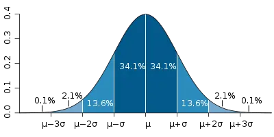
Considering mean=0, and S.D=1,

From the above figure, it is evident that the bell curve is symmetric about its mean. For, one standard deviation i.e., sigma=1, 34.1% of the data falls under this region.

• For -1<sigma<1, 68.2 % of the data falls within this region.
• For -2<sigma<2, 95.4 % of the data falls within this region.
• For -3<sigma<3, 99.6 % of the data falls within this region.