Basics of ML & AL
Tasks
1)Calculate all 4 business moments using pen and paper for the below data set?
2)What is the significance of expected value when simple mean (Sum of all observations/number of observations) is already in place
3)Having skewness in the curve considered to be bad in the analysis?
4)Evaluate the probabilities for continuous normal distribution with given mean = 680 and standard deviation = 31
a)P(X<711)
b)P(X>740)
c)P(600<x<720)
d)P(X=720)
5)Explain the curve on the right side
Task 1
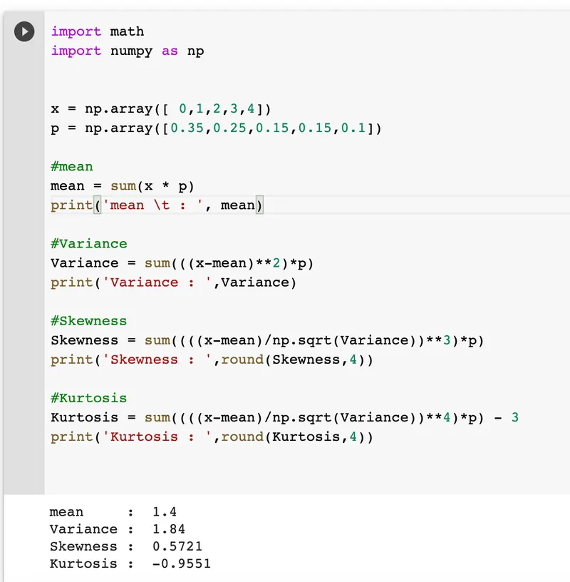
Calculate all 4 business moments using the python program for the below data set?
Task 2
What is the significance of expected value when simple mean (Sum of all observations/number of observations) is already in place
The Expected value of a discrete random variable, X indicates the average value and is denoted as E(X). The expected value for a random variable is its mean. It is the value that you would expect to obtain if you conduct an experiment whose outcomes are represented by the random variable. It is the weighted average of all the possible values where the probabilities of occurrence of the variables are the weights. For a discrete random variable, the probabilities of each random variable are the weights whereas, for a continuous random variable, the values of the probability density function are the weights. In Probability theory, the expected value of a random variable is the value you would expect to obtain if the random variable process was repeated an infinite number of times and the average of those values were taken.
The mean of a data set is exactly the same by definition and concept as the expectation and mainly differs in the application. When we have a data set along with its frequencies, then we use the mean formula to calculate the average. By summing up the product of the random variable with its frequency and dividing by the total frequency, we get the average value. If instead, we had a data set with the probabilities of occurrence for each random variable, then we would use the expectation formula to determine the average. Also, if the probabilities for all of the random variables are equal, then we can find the average using the mean directly instead of the expectation. Both are the same conceptually because the frequency of a variable occurring is the same as its probability of occurrence.
For instance, for the above data set, we are given the probabilities of the random variable, X. Suppose, we had a sample data of 100 values. Then the frequency of each variable would be the probability multiplied by 100. E.g. for X = 0, the frequency would be 35, X = 1, the frequency would be 25. The probability of each variable was determined by knowing how frequently the variable occurred and divided by the total number of trials. So for 100 trials, if X = 1 occurred 35 times, its probability would be 0.35 which is how the probability values are obtained in the table.
If we used the frequencies and tried to sum the products of the variable and their respective frequencies, we would get a value of 140. Since the total frequency is 100 (100 trials), then the mean would be 140/100 = 1.4, which is the same as the expectation, E(X).
Task 3
Having skewness in the curve considered to be bad in the analysis?
Skewness is defined as the measure of the symmetry (or lack of symmetry) of a data set. Having skewness is neither good nor bad. It simply describes the distribution from a value. Whether skewness is good or bad is dependent on the application of the data.
For a normal distribution, the measures of central tendency (mean, median and mode) are equal to each other whereas, for a skewed distribution, the measures are scattered. For instance, if a distribution is positively skewed, the mean would be found to the right side and conversely to the left side for that of a negatively skewed distribution. This can be inconvenient when locating these measures for analysis.
Also, when statistical tests are performed, misleading results can be obtained from data that is highly skewed. In order to overcome this effect, data transformation tools are used to bring the distribution more closely to resemble a normal one.
But in general, skewness is neither good nor bad without identifying the application of the data or the purpose for what it was obtained. Different applications have different meanings for skewed or non-skewed data.
A distribution can have a positive skew, no skew or a negative skew or even be undefined. Each instance is shown in the image below with the general shape of the distribution curve.
The above image shows the 3 basic possibilities for the skew in a distribution of data.
A negatively skewed distribution will be skewed to the left and most of the values are gathered at the right tail of the distribution. This distribution will have a negative skewness coefficient. Normal distribution will have pure symmetry and is not skewed either to the left or the right. It will have a skewness coefficient of 0. A positively skewed distribution will be skewed to the right and most of the values are gathered at the left tail of the distribution. This will have a positive skewness coefficient.
The general rule of thumb is that:
If the skewness is between -0.5 and 0.5, the distribution curve is considered to have no skew (perfect symmetry).
If the skewness is between -1 and -0.5 or 0.5 and 1, the skew of the distribution curve (whether positive or negative) is moderate.
If the skewness is lower than -1 or higher than 1, then the skew of the distribution curve (whether positive or negative) is quite high.
Task 4
Evaluate the probabilities for continuous normal distribution with
given mean = 680 and
standard deviation = 31
a)P(X<711)
b)P(X>740)
c)P(600<x<720)
d)P(X=720)
The "z-score formula":
z = (x − μ)/σ
The value of μ is 680
The value of σ is 31
a) P(X<711)
The value of x is 711
then, Z score is
Z= 711-680/31
= 1
From the Z table
P(Z<1) = 0.8413
This is the area to the left of the Z score since X is less than 711.
b) P(X>740)
The value of x is 740
then, Z score is
Z=740-680/31
=1.935
P(Z<1.935)=0.9713
This is the area to the left of the Z score, but we need to calculate the area to the right of the Z score.
Now,
P(Z>1.935)=1-P(Z<1.935)
=1-0.9713
=0.0287
The area to the right of the Z score gives the value of 0.0287 which is 2.87% of probability P(X>740)
c)P(600<X<720)
Z=600-680/31
=-2.58
Z=720-680/31
=1.29
We have to find the area for Z score -2.58 and 1.29 and subtract the value to get the probability P(-2.58<Z<1.29)
P(-2.58<Z<1.29)=0.90147 - 0.00466
P(-2.58<Z<1.29) = 0.89681
89.6% of are between P(600<X<720)
d)P(X=720)
Z=720-680/31
=1.29
P(Z = 1.29) = 0.9015 - 0.9015 = 0
Task 5
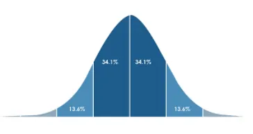
Explain the curve on the right side
The bell curve sometimes referred to as a normal curve, is a way of graphically displaying normally distributed data. What is normally distributed data? It's a data set with an identical mean, median, and mode. Put more simply, normally distributed data has a perfect average. Look at a bell curve and you'll see it is perfectly symmetrical. There is exactly 50% of the data on either side of the midpoint. You'll also notice that the largest amount is at the centre of the curve and it tapers off as it gets higher and lower, giving it the distinctive bell shape.
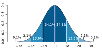 |
The beauty of the bell curve, and why it is so important to understand, is that the information it displays has certain characteristics. As mentioned above, the average of the data is perfectly in the middle, but you can also see there are percentages given for each 'chunk' of data. Each one of these data chunks represents one standard deviation, but don't worry about that term for now. Just think of them as chunks of data. In a bell curve of normally distributed data, those percentages given will always be true. The middle chunk will always add up to 68.2%, the next chunk is 27.2%, the next is 4.2%, and the last little bit is 0.2%. Note that because of rounding, they don't add up to 100%.
It is important to note here that this is true only for perfectly normal data. You may encounter graphs that look like a bell curve but the data isn't perfectly normal. In other words, the graph won't be perfectly symmetrical and it doesn't have identical mean, median, and mode. This is what we call an approximately normal data set. These are usually quite close to a bell curve, and sometimes you can get away with using these bell curve 'chunk' percentages, but know that they won't be super accurate unless the data is perfectly normal.