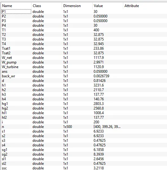
BASIC RANKINE CYCLE SIMULATOR

AIM: TO SIMULATE BASIC RANKINE CYCLE

OBJECTIVES:

1. Creating a Rankine Cycle Simulator using OCTAVE/MATLAB. Calculating the state points of the Rankine Cycle based on user inputs.

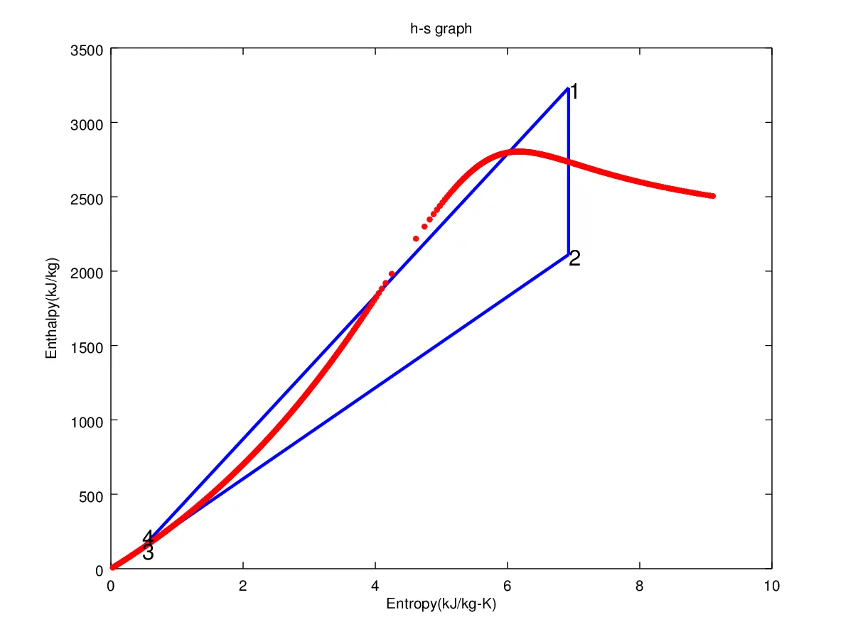
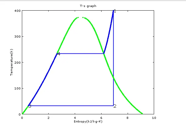
2.Then, plotting the corresponding T-s and h-s plots for the given set of inputs.

RANKINE CYCLE DESCRIPTION:

The Rankine cycle is the fundamental operating cycle of all power plants where an operating fluid is continuously evaporated and condensed. The selection of operating fluid depends mainly on the available temperature range.

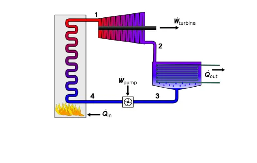
The different processes here are :

PROCESS 1-2 : Isentropic Expansion in the turbine

PROCESS 2-3 : Isobaric Heat Rejection by the condenser

PROCESS 3-4 : Isentropic Compression in the pump

PROCESS 4-1 : Isobaric Heat Addition by the boiler

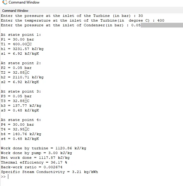
Here the Given Input Values are:

Turbine Inlet temperature = 400° C

Turbine Inlet Pressure = 30 bars

Turbine Outlet Pressure = 0.05 bars = Condenser Inlet Pressure

MAIN CODE:

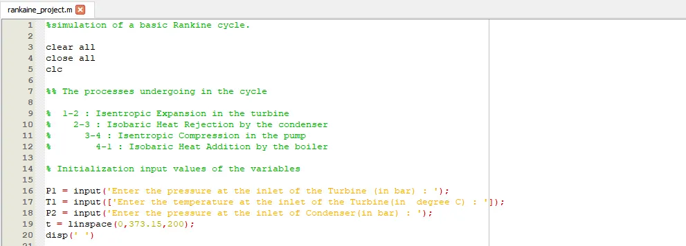
%simulation of a basic Rankine cycle.

clear all
close all
clc

%% The processes undergoing in the cycle

%  1-2 : Isentropic Expansion in the turbine
%    2-3 : Isobaric Heat Rejection by the condenser
%      3-4 : Isentropic Compression in the pump
%        4-1 : Isobaric Heat Addition by the boiler

% Initialization input values of the variables 

P1 = input('Enter the pressure at the inlet of the Turbine (in bar) : ');
T1 = input(['Enter the temperature at the inlet of the Turbine(in  degree C) : ']);
P2 = input('Enter the pressure at the inlet of Condenser(in bar) : ');
t = linspace(0,373.15,200);
disp(' ')


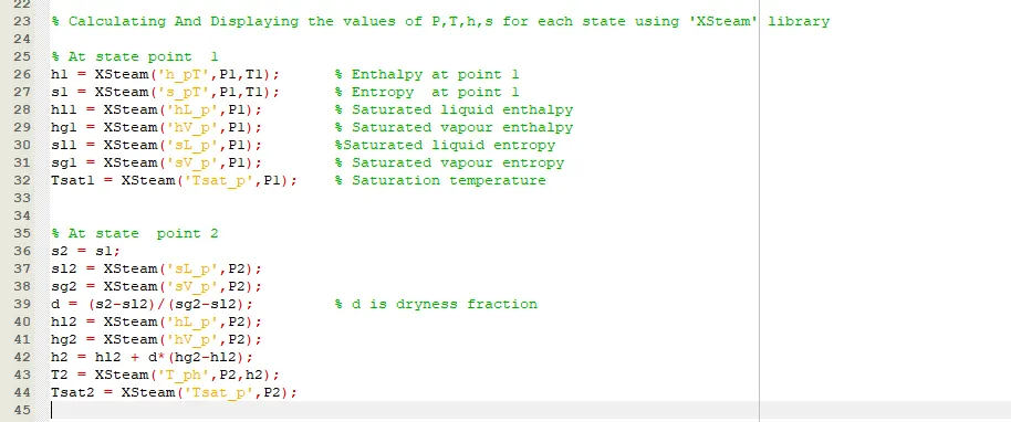
% Calculating And Displaying the values of P,T,h,s for each state using 'XSteam' library

% At state point  1
h1 = XSteam('h_pT',P1,T1);      % Enthalpy at point 1
s1 = XSteam('s_pT',P1,T1);      % Entropy  at point 1
hl1 = XSteam('hL_p',P1);        % Saturated liquid enthalpy
hg1 = XSteam('hV_p',P1);        % Saturated vapour enthalpy
sl1 = XSteam('sL_p',P1);        %Saturated liquid entropy
sg1 = XSteam('sV_p',P1);        % Saturated vapour entropy
Tsat1 = XSteam('Tsat_p',P1);    % Saturation temperature


% At state  point 2
s2 = s1;
sl2 = XSteam('sL_p',P2);
sg2 = XSteam('sV_p',P2);
d = (s2-sl2)/(sg2-sl2);         % d is dryness fraction
hl2 = XSteam('hL_p',P2);
hg2 = XSteam('hV_p',P2);
h2 = hl2 + d*(hg2-hl2);
T2 = XSteam('T_ph',P2,h2);
Tsat2 = XSteam('Tsat_p',P2);



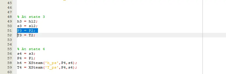
% At state 3
h3 = hl2;
s3 = sl2;
P3 = P2;
T3 = T2;


% At state 4
s4 = s3;
P4 = P1;
h4 = XSteam('h_ps',P4,s4);
T4 = XSteam('T_ps',P4,s4);

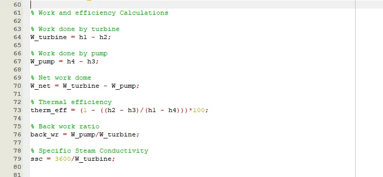
% Work and efficiency Calculations

% Work done by turbine
W_turbine = h1 - h2;

% Work done by pump
W_pump = h4 - h3;

% Net work dome
W_net = W_turbine - W_pump;

% Thermal efficiency
therm_eff = (1 - ((h2 - h3)/(h1 - h4)))*100;

% Back work ratio
back_wr = W_pump/W_turbine;

% Specific Steam Conductivity
ssc = 3600/W_turbine;


%% Plotting Of Different curevs


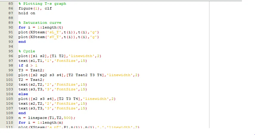
% Plotting T-s graph
figure(1), clf
hold on

% Saturation curve
for i = 1:length(t)
plot(XSteam('sL_T',t(i)),t(i),'g')
plot(XSteam('sV_T',t(i)),t(i),'g')
end

% Cycle
plot([s1 s2],[T1 T2],'linewidth',2)
text(s1,T1,'1','FontSize',15)
if d > 1
T3 = Tsat2;
plot([s2 sg2 s3 s4],[T2 Tsat2 T3 T4],'linewidth',2)
T2 = Tsat2;
text(s2,T2,'2','FontSize',15)
text(s3,T3,'3','FontSize',15)
else
plot([s2 s3 s4],[T2 T3 T4],'linewidth',2)
text(s2,T2,'2','FontSize',15)
text(s3,T3,'3','FontSize',15)
end
n = linspace(T1,T2,500);
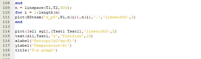
for i = 1:length(n)
plot(XSteam('s_pT',P1,n(i)),n(i),'.','linewidth',2)
end

plot([sl1 sg1],[Tsat1 Tsat1],'linewidth',2)
text(sl1,Tsat1,'4','FontSize',15)
xlabel('Entropy(kJ/kg-K)')
ylabel('Temperature(k)')
title('T-s graph')


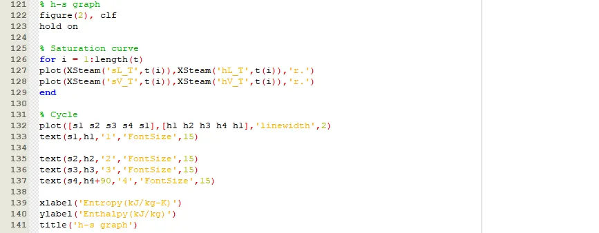
% h-s graph
figure(2), clf
hold on

% Saturation curve
for i = 1:length(t)
plot(XSteam('sL_T',t(i)),XSteam('hL_T',t(i)),'r.')
plot(XSteam('sV_T',t(i)),XSteam('hV_T',t(i)),'r.')
end

% Cycle
plot([s1 s2 s3 s4 s1],[h1 h2 h3 h4 h1],'linewidth',2)
text(s1,h1,'1','FontSize',15)

text(s2,h2,'2','FontSize',15)
text(s3,h3,'3','FontSize',15)
text(s4,h4+90,'4','FontSize',15)

xlabel('Entropy(kJ/kg-K)')
ylabel('Enthalpy(kJ/kg)')
title('h-s graph')

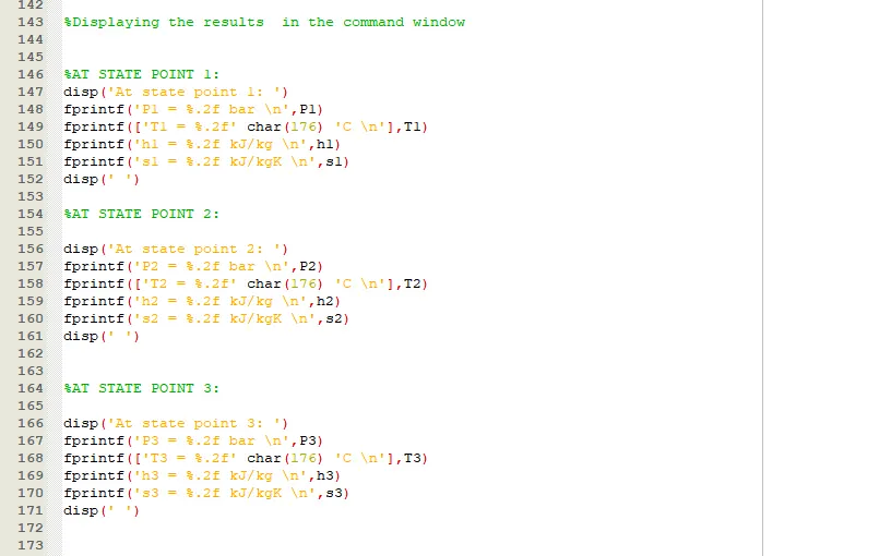
%Displaying the results  in the command window


%AT STATE POINT 1:
disp('At state point 1: ')
fprintf('P1 = %.2f bar \n',P1)
fprintf(['T1 = %.2f' char(176) 'C \n'],T1)
fprintf('h1 = %.2f kJ/kg \n',h1)
fprintf('s1 = %.2f kJ/kgK \n',s1)
disp(' ')

%AT STATE POINT 2:

disp('At state point 2: ')
fprintf('P2 = %.2f bar \n',P2)
fprintf(['T2 = %.2f' char(176) 'C \n'],T2)
fprintf('h2 = %.2f kJ/kg \n',h2)
fprintf('s2 = %.2f kJ/kgK \n',s2)
disp(' ')


%AT STATE POINT 3:

disp('At state point 3: ')
fprintf('P3 = %.2f bar \n',P3)
fprintf(['T3 = %.2f' char(176) 'C \n'],T3)
fprintf('h3 = %.2f kJ/kg \n',h3)
fprintf('s3 = %.2f kJ/kgK \n',s3)
disp(' ')


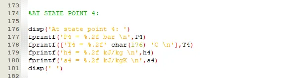
%AT STATE POINT 4:

disp('At state point 4: ')
fprintf('P4 = %.2f bar \n',P4)
fprintf(['T4 = %.2f' char(176) 'C \n'],T4)
fprintf('h4 = %.2f kJ/kg \n',h4)
fprintf('s4 = %.2f kJ/kgK \n',s4)
disp(' ')


fprintf('Work done by turbine = %.2f kJ/kg \n', W_turbine)
fprintf('Work done by pump = %.2f kJ/kg \n', W_pump)
fprintf('Net work done = %.2f kJ/kg \n', W_net)
fprintf('Thermal efficiency = %.2f %% \n', therm_eff)
fprintf('Back-work ratio = %f \n', back_wr)
fprintf('Specific Steam Conductivity = %.2f kg/kWh \n',ssc)

Similarly at the state points 3 and 4 same were calculated.

STEP 3: In this step using basic relations between work and physical parameters and "basic mathematical operations in octave" the "W_net" , "back_wr" etc. were calculated.

STEP 4: This step was to plot the T-s curve . Here again we used the provided "XSteam" library function to plot the T-s Curve at different temperature array values.

Then along with the state points the curve was plotted.

STEP 5: Similarly In this step the T-s curve was plotted. Here again we used the provided "XSteam" library function to plot the h-s Curve at different temperature array values.

Then along with the state points the curve was plotted.

STEP 6: In this step the values of physical parameters at the state points were displayed in the output window. This was done for all the "4" defining state points in similar way.

STEP 7: In this step The final results i.e. "W_net" "W_turbine" "W-pump" "back_wr" "ssc" "therm_eff" were printed.