EFFECT OF INITIAL PRESSURE AND TEMPERATURE ON IGNITION DELAY OF METHANE-AIR COMBUSTION USING CANTERA IN PYTHON

Aim :

1. To understand the effect of initial pressure and initial temperature on auto ignition time delay
2. To understand how species concentration is going to vary wrt to time for a particular pressure and temperature

Introduction :

The fuel air mixture can automatically combust if it attains proper environment to do so. It depends on temperature pressure and Equivalence ratio of mixture etc. The lowest temperature at a given environment settings when the fuel air mixture ignites by itself is called Auto ignition temperature

This temperature is required to supply the activation energy needed for combustion. The time between attaining the temperature and starting the combustion is called Ignition delay. This time is usually in milli seconds

Reactor in cantera :

A cantera reactor is the simplest reacting system that can be created. The reactor has a volume and within the reactor there are no gradients in composition and other thermodynamic properties. The reactor just defines the governing equations to be solved and the time integration is performed on the reactor network. Even for a single reactor a reactor network is required. The advance method is used to integrate the reactor network, i.e when the advance method is called the reactor state changes.

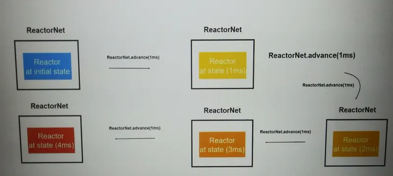
Python code for the effect of initial pressure on ignition delay :

'''
Program to find the effect of initial pressure  on Ignition delay of Methane-Air combustion

CH4 + 2(O2+ 3.76N2) -------> CO2 + 2H2O + 7.52N2 (Stoichiometric reaction)

Author : Harshith Rajamahanti

'''
import sys
import numpy as np
import cantera as ct
import matplotlib.pyplot as plt

gas = ct.Solution('gri30.cti')

T_initial=1250  #Temp in kelvin
p_low=1*101325  # Lower limit of pressure in pascal
p_high=5*101325 # Upper limit of pressure in pascal
dp = 0.5*101325 # Step size of pressure 
p_value=np.arange(p_low,p_high+dp,dp)

Auto_ig_temp=[]
Auto_ig_time=[]

# Loop for different pressure values 

for i in range(0,len(p_value)):
	gas.TPX=T_initial,p_value[i],{'CH4':1,'O2':2,'N2':7.52}
	r=ct.IdealGasReactor(gas)
	sim=ct.ReactorNet([r])
	time=0.0
	states=ct.SolutionArray(gas,extra=['t_ms','t'])
	count=0

	for n in range(10000):
		time=time+1e-3
		sim.advance(time)
		states.append(r.thermo.state,t_ms=time*1e3,t=time)

		if(states.T[n]>=(T_initial+400))and count==0:
			Auto_ig_temp.append(states.T[n])
			Auto_ig_time.append(states.t_ms[n])
			print(n)
			count=1

	plt.figure(1)
	plt.plot(states.t_ms,states.T)

plt.figure(1)
plt.xlabel('Time in ms')
plt.ylabel('Temperature in k')
plt.title('Temperature vs time')
plt.grid(True)
plt.minorticks_on()
plt.grid(which='minor',alpha=0.2)
plt.legend(['p_initial= '+ str(p)+' (atm)' for p in p_value/101325])
plt.show()

plt.figure(2)
plt.plot(p_value/101325,Auto_ig_time,'-o')
plt.xlabel('Initial pressure in atm')
plt.ylabel('Ignition delay in ms')
plt.title('Effect of initial pressure of mixture on Ignition delay time')
plt.grid(True)
plt.minorticks_on()
plt.grid(which='minor',alpha=0.2)
plt.show()

Code explanation :

1. Importing all the important packages required for the code
2. Initial temperature is taken as 1250 K and the initial pressure is varied from 1 atm to 5 atm
3. 1 st For loop is for pressure i.e it runs for the pressures of 1 atm to 5 atm with an interval of 0.5 i.e the loop runs for 10 times
4. The initial temperature(fixed), initial pressure(varied in for loop) and the mole fraction properties are passed to the gas object
5. The gas object is then passed to 'IdealGasReactor' which is then passed on to 'ReactorNet'
6. The 'states' variable gives the values of the solution by means of 'SolutionArray'
7. The 2nd For loop is for time. The loop runs for 10,000 times with a time step of 1e-3 i.e the simulation os done for 10 sec or 10,000 milli sec
8. The cantera software simulates the combustion using its own time step till the 'time', which we pass as an argument to 'advance' method
9. The states object is now appended with the new values of Reactor 'r' object
10. If Loop inside the 2nd For loop is to calculate Auto-Ignition Temperature and Ignition Delay time. If the temperature is greater than or equal to initial temperature + 400 K its the Auto Ignition temperature and n value represents the array index. If the Ignition time has to be calculated for a particular pressure value the time in milli sec will be equal to 'n+1'
11. States.T gives the Temperature values in the form of arrays at each and every time step
12. For every value of Pressure there will be a single value of Ignition delay so here 10 ignition delay values will be displayed.
13. Then required parameters are plotted on time scale.

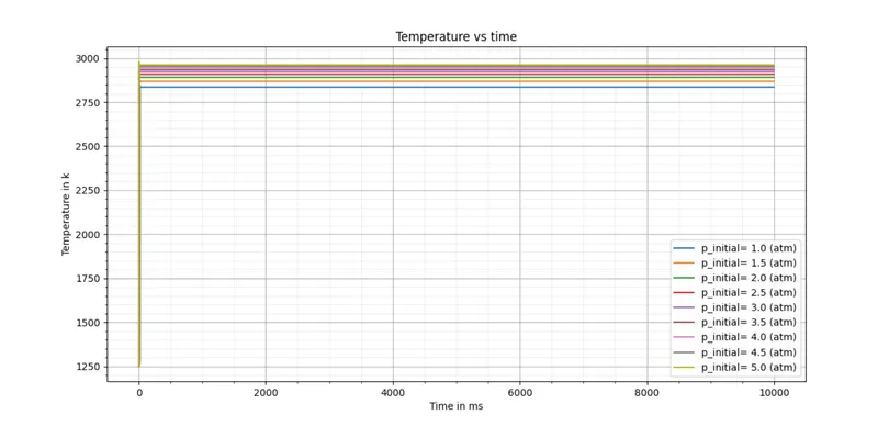
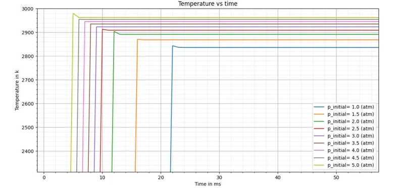
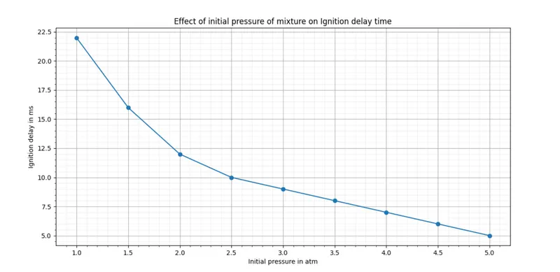
Python code for the effect of initial temperature on ignition delay :

'''
Program to find the effect of initial temperature on Ignition delay of Methane-Air combustion

CH4 + 2(O2+ 3.76N2) -------> CO2 + 2H2O + 7.52N2 (Stoichiometric reaction)

Author : Harshith Rajamahanti

'''
import sys
import numpy as np
import cantera as ct
import matplotlib.pyplot as plt

gas = ct.Solution('gri30.cti')

p_initial=5*101325  #Temp in kelvin
T_low=950  # Lower limit of temperature in kelvin
T_high=1450 # Upper limit of temperature in kelvin
dt = 100 # Step size of pressure 
T_value=np.arange(T_low,T_high+dt,dt)

Auto_ig_temp=[]
Auto_ig_time=[]

# Loop for different temperature values 

for i in range(0,len(T_value)):
	gas.TPX=T_value[i],p_initial,{'CH4':1,'O2':2,'N2':7.52}
	r=ct.IdealGasReactor(gas)
	sim=ct.ReactorNet([r])
	time=0.0
	states=ct.SolutionArray(gas,extra=['t_ms','t'])
	count=0

	for n in range(10000):
		time=time+1e-3
		sim.advance(time)
		states.append(r.thermo.state,t_ms=time*1e3,t=time)

		if(states.T[n]>=(T_value[i]+400))and count==0:
			Auto_ig_temp.append(states.T[n])
			Auto_ig_time.append(states.t_ms[n])
			print(n)
			count=1

	plt.figure(1)
	plt.plot(states.t_ms,states.T)

plt.figure(1)
plt.xlabel('Time in ms')
plt.ylabel('Temperature in k')
plt.title('Temperature vs time')
plt.grid(True)
plt.minorticks_on()
plt.grid(which='minor',alpha=0.2)
plt.legend(['T_initial= '+ str(T)+' (K)' for T in T_value])
plt.show()


plt.figure(2)
plt.plot(T_value,Auto_ig_time,'-o')
plt.xlabel('Initial temperature in K')
plt.ylabel('Ignition delay in ms')
plt.title('Effect of initial temperature of mixture on Ignition delay time')
plt.grid(True)
plt.minorticks_on()
plt.grid(which='minor',alpha=0.2)
plt.show()

Code explanation :

1. Importing all the important packages required for the code
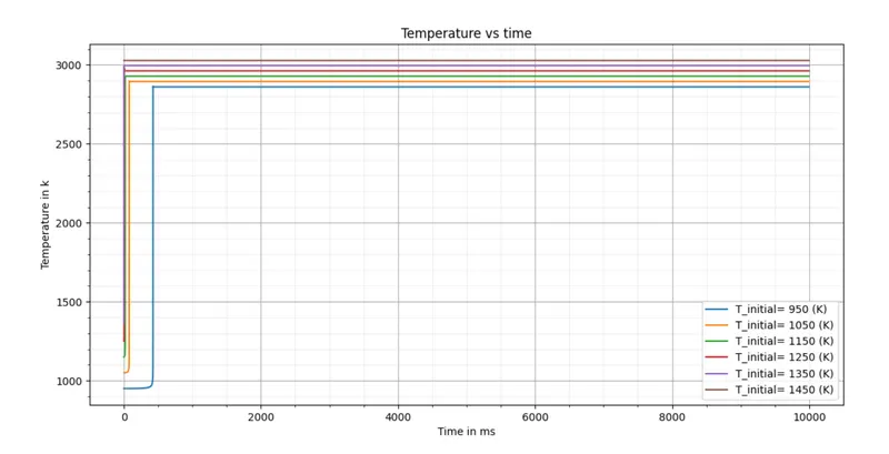
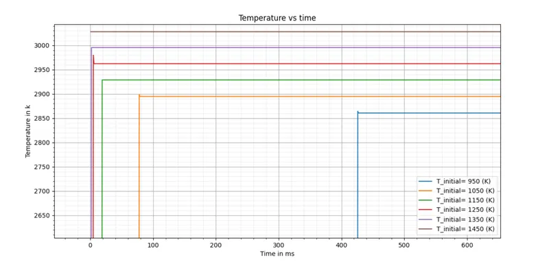
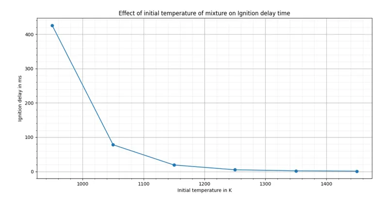
2. Initial pressure is taken as 5 atm and the initial temperature is varied from 950 K to 1450 K
3. 1 st For loop is for temperature i.e it runs for the temperatures of 950 K to 1450 K with an interval of 100 i.e the loop runs for 6 times
4. The initial pressure(fixed), initial temperature(varied in for loop) and the mole fraction properties are passed to the gas object
5. The gas object is then passed to 'IdealGasReactor' which is then passed on to 'ReactorNet'
6. The 'states' variable gives the values of the solution by means of 'SolutionArray'
7. The 2nd For loop is for time. The loop runs for 10,000 times with a time step of 1e-3 i.e the simulation os done for 10 sec or 10,000 milli sec
8. The cantera software simulates the combustion using its own time step till the 'time', which we pass as an argument to 'advance' method
9. The states object is now appended with the new values of Reactor 'r' object
10. If Loop inside the 2nd For loop is to calculate Auto-Ignition Temperature and Ignition Delay time. If the temperature is greater than or equal to initial temperature + 400 K its the Auto Ignition temperature and n value represents the array index. If the Ignition time has to be calculated for a particular pressure value the time in milli sec will be equal to 'n+1'
11. States.T gives the Temperature values in the form of arrays at each and every time step
12. For every value of temperature there will be a single value of Ignition delay so here 6 ignition delay values will be displayed.
13. Then required parameters are plotted on time scale.

Python code for Species concentration variation wrt to time :

'''
Program to find the variation of species concentration wrt to time for Methane-Air combustion

CH4 + 2(O2+ 3.76N2) -------> CO2 + 2H2O + 7.52N2 (Stoichiometric reaction)

Author : Harshith Rajamahanti

'''
import sys
import numpy as np
import cantera as ct
import matplotlib.pyplot as plt

gas = ct.Solution('gri30.cti')

P=5*101325 # pa
T=1000     # k

gas.TPX=T,P,{'CH4':1,'O2':2,'N2':7.52}
r=ct.IdealGasReactor(gas)
sim=ct.ReactorNet([r])
time=0.0
states=ct.SolutionArray(gas)
temp_state=[]
time_state=[]

for n in range(10000):
	time=time+1e-3
	sim.advance(time)
	states.append(r.thermo.state)
	temp_state.append(states.T[n])
	time_state.append(time)

CH4_species=states.X[:,gas.species_index('CH4')]
O2_species=states.X[:,gas.species_index('O2')]
N2_species=states.X[:,gas.species_index('N2')]
CO2_species=states.X[:,gas.species_index('CO2')]
H2O_species=states.X[:,gas.species_index('H2O')]
CO_species=states.X[:,gas.species_index('CO')]
OH_species=states.X[:,gas.species_index('OH')]

fig1,a1=plt.subplots(2,4)
plt.suptitle('Temperature and Molefractions for reaction at 1000 K and 5 bar')

a1[0,0].plot(time_state,temp_state)
a1[0,0].set_title('Temperature')
a1[0,0].set_xlabel('Time in sec')
a1[0,0].set_ylabel('Temperature in K')
a1[0,0].grid('both')

a1[0,1].plot(time_state,CH4_species)
a1[0,1].set_title('CH4 Mole Fraction')
a1[0,1].set_xlabel('Time in sec')
a1[0,1].grid('both')

a1[0,2].plot(time_state,O2_species)
a1[0,2].set_title('O2 Mole Fraction')
a1[0,2].set_xlabel('Time in sec')
a1[0,2].grid('both')

a1[0,3].plot(time_state,N2_species)
a1[0,3].set_title('N2 Mole Fraction')
a1[0,3].set_xlabel('Time in sec')
a1[0,3].grid('both')

a1[1,0].plot(time_state,CO2_species)
a1[1,0].set_title('CO2 Mole Fraction')
a1[1,0].set_xlabel('Time in sec')
a1[1,0].grid('both')

a1[1,1].plot(time_state,H2O_species)
a1[1,1].set_title('H2O Mole Fraction')
a1[1,1].set_xlabel('Time in sec')
a1[1,1].grid('both')

a1[1,2].plot(time_state,CO_species)
a1[1,2].set_title('CO Mole Fraction')
a1[1,2].set_xlabel('Time in sec')
a1[1,2].grid('both')

a1[1,3].plot(time_state,OH_species)
a1[1,3].set_title('OH Mole Fraction')
a1[1,3].set_xlabel('Time in sec')
a1[1,3].grid('both')

plt.show()

Code explanation :

1. Importing all the important packages required for the code
2. Initial temperature is taken as 1000 K and initial pressure is taken as 5 atm
3. The initial pressure(fixed), initial temperature(fixed) and the mole fraction properties are passed to the gas object
4. The gas object is then passed to 'IdealGasReactor' which is then passed on to 'ReactorNet'
5. The 'states' variable gives the values of the solution by means of 'SolutionArray'
6. The For loop is for time. The loop runs for 10,000 times with a time step of 1e-3 i.e the simulation os done for 10 sec or 10,000 milli sec
7. The cantera software simulates the combustion using its own time step till the 'time', which we pass as an argument to 'advance' method
8. States.T gives the Temperature values in the form of arrays at each and every time step
9. Major species are choosen and its concentration at each and every time step is evaluated
10. Then required parameters are plotted on time scale

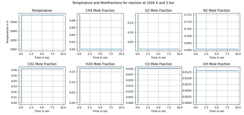
As the initial temperature was 1000 K, the mixture was likely to auto ignite and it did ignite. This took the temperature to approximately 2800 K . CH4 molefraction went to 0. CO2 and H2O mole fraction increased from 0.The N2 mole fraction was expected not to change but it changed because it might have formed NOX. O2 mole fraction reduced to some value but not to 0. OH and CO mole fractions are also present at the end.

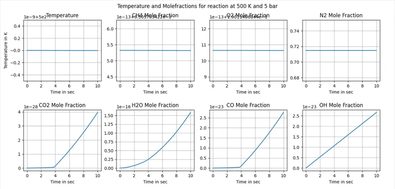
The Auto ignition temperature of Methane at 1 atm is around 873 K. The initial temperature was 500 K which is less than the auto ignition temperature so no combustion takes place. Due to this the temperature and mole fraction did not change as much.

Conclusion :

1. With increase in initial pressure Ignition delay decreases but it is not always true the exact variation is determined by sensitivity analysis.
2. With increase in initial temperature Ignition delay first decreases to some extent and then it increases which is called 'Negative temperature coefficient'(NTC) and later it decreases.
3. If the initial temperature is less than the Auto ignition temperature combustion doesn't takes place