Frontal Crash Simulation

Frontal Crash Simulation
OBJECTIVE: Simulate a Frontal car crash simulation of Dodge Neon BIW using RADIOSS solver and Preprocessing using HyperMesh / HyperCrash.

• To perform the crash analysis on the frontal section of the car and to check where the stresses are acting on it.
• To check the unit systems and change if necessary
• Create an interface of Type 7 with the friction value of 0.2 and other parameters.
• Make sure there aren’t any penetrations
• Correct rigid bodies for any issues
• Create a rigid wall with friction 0.1.
• Compare the model weight with the full-scale 300k nodes model and use added masses to reach the target weight of 700kg while getting CG about the required range.
• Give an initial velocity of 35 mph.
• Use a model checker to ensure good quality.
• Give the Time-step: 0.5 microseconds.
• Give Run time as 80 ms.

Output Deliverables:

• Sectional force in the rails at the location of indicated node 174247.
• The axial force received on the rails from the bumper.
• Shotgun cross-sectional forces.
• A pillar cross-section.
• Acceleration curve received on the accelerometer at base of B pillar (on B pillar rocker).
• Intrusions on the dash wall 66695,66244

ABSTRACT:

The objective of a crash test for Federal Motor Vehicle Safety Standard (FMVSS) No. 208 is to measure how well a passenger vehicle would protect its occupants in the event of a serious real-world frontal crash. This is sometimes referred to as the crashworthiness of a vehicle. This report reviews potential test procedures for evaluating frontal crashworthiness.

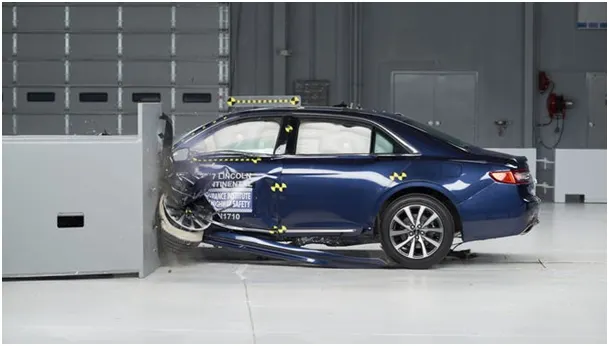
The ideal frontal crash test procedure will be able to evaluate occupant protection while ensuring that the vehicle will not jeopardize its crash “friendliness” with its collision partners. Finally, the test conditions (e.g., impact speed, impact angle, and test device) must be representative of the frontal crash environment to which passenger vehicles are exposed on the highway. The objective of a crash test for Federal Motor Vehicle Safety Standard (FMVSS) No. 208 is to measure the crashworthiness of a passenger vehicle. The standard specifies performance requirements for the protection of vehicle occupants in crashes. Historically, this has encouraged improvements to the vehicle structure and restraint systems to enhance occupant crash protection.

• The frontal impact is performed at 64kph (40mph), the car crashes into a deformable barrier with 40% of its width front on the driver side (offset). Readings taken from the crash test dummies are used to assess protection given to adult occupants in the front seat.
• Each car tested is subjected to an offset impact into an immovable block fitted with a deformable aluminum honeycomb face.
• This impact is intended to replicate the effect caused in the car when crashing 55km/h 50% offset frontal crash with a similar mass car. As most frontal crashes involve only part of each car's front, the test is offset to replicate a half-width frontal impact between two cars.
• In the test, this is replicated by having 40 percent of the width of the car crashing into the aluminium deformable barrier. This represents the most frequent type of road crash, resulting in serious or fatal injury.
• The barrier face is deformable to represent the deformable nature of the cars. Two adult dummies are placed representing average size men in the driver's seat and front passenger and two children, aged 18 months and 3 years old, on child restraint systems are placed in the rear seat.
• Contact between the occupant and hard and intruding parts of the passenger compartment is the main cause of serious and fatal injuries for restrained adult car occupants.
• The test speed of 64 km/h represents a car-to-car collision with each car traveling at around 55 km/h and crashing 50% of their width.
• The difference in speed is due to the energy absorbed by the deformable face. Accident research has shown that this impact speed covers a significant proportion of serious and fatal accidents.
• By preventing intrusion, the chances of the occupant impacting the car's interior are minimized with space remaining for the restraint system to operate effectively. Steering wheel and dashboard-mounted airbags are an important part of the driver's restraint system.

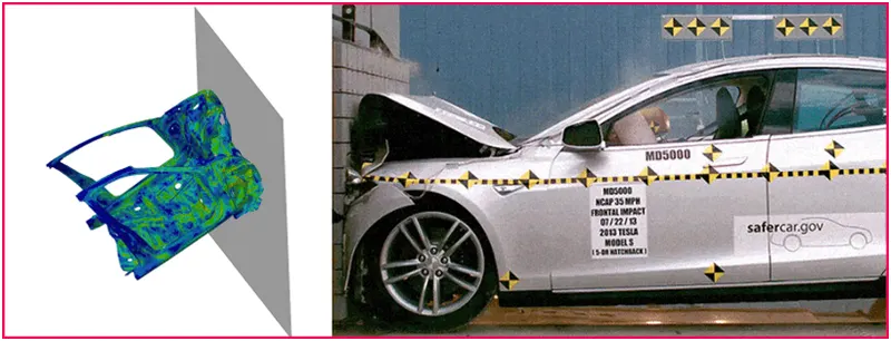
Crashworthiness Requirements

The vehicle structure should be sufficiently stiff in bending and torsion for proper ride and handling. It should minimize high-frequency fore-aft vibrations that give rise to harshness. In addition, the structure should yield a deceleration pulse that satisfies the following requirements for a range of occupant sizes, ages, and crash speeds for both genders: Deformable, yet stiff, front structure with crumple zones to absorb the crash kinetic energy resulting from frontal collisions by plastic deformation and
prevent intrusion into the occupant compartment, especially in case of offset crashes and collisions with narrow objects such as trees.

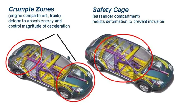
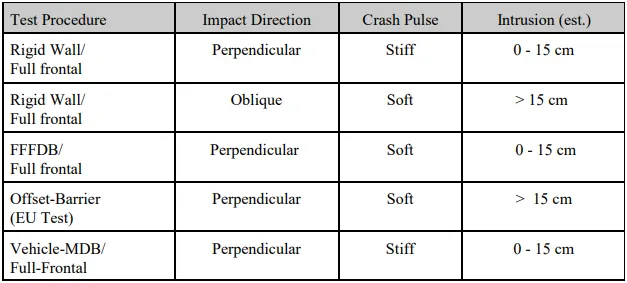
• Short vehicle front ends, driven by styling considerations, present a challenging task to the crash-worthiness engineer.
• Deformable rear structure to maintain the integrity of the rear passenger compartment and protect the fuel tank.
• Properly designed side structures and doors to minimize intrusions in side-impact and prevent doors from opening due to crash loads.
• Strong roof structure for rollover protection.
• Properly designed restraint systems that work in harmony with the vehicle structure to provide the occupant with an optimal ride down and protection in different interior spaces and trims.
• Accommodate various chassis designs for different power train locations and drive configurations.

PROCEDURE:
Set-up has to be followed,

• First, we want to import the neo
• Check for UNIT SYSTEM
• Import model in HYPER CRUSH
• Check for penetration and intersection
• Add masses to reach a target weight of 700kg
• Export changes file and import in HYPER MESH
• Create Interface contact's
• Create interface contact between component and bumper
• Create a rigid wall
• Add velocity to the nodes
• Create cross-section's
• Create acceleration nodes
• Create springs to check deflection
• Assign property to springs
• Create TH for section forces, intrusion springs, interface contacts
• Create cards
• Model checker
• n_front file by using the import option and select the file that we want to import the data of file name as neon_front_0000.rad that is referred to as an input file of the simulation and click import. Now the file is imported and the import selection process and import file dialog box is shown below,

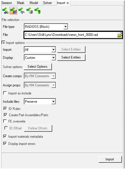
Fig: Import Dialog box

After importing, the input file a model will open.

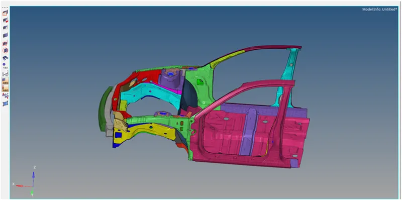
Fig: Open model

• Now check the unit system and verify that the same pattern of the unit system has followed in this simulation. It could be in either [Mg mm s] or [Kg mm ms] that are mentioned by the instructor.

• The unit system is required to obtain the resultant plots in that certain units. The unit system for this simulation is shown below,

After verifying the unit system to create an appropriate interface with the friction of 0.2 and using recommended parameters, Here there should be a default interface is present in the model that is shown below,

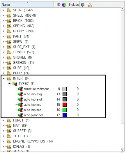
Fig: Solver table

• We are deleting the default interface(TYPE-7) that is present in this model because it indicates the group of different sectors of self contact in the vehicle. we want to create the total self contact of the BIW body of the vehicle.
• Therefore create the interface of Type-7 by selecting the solver>inter>right click inter>select create and enter the recommended parameters in that properties card. Type-7 interface is used because it is nodes to surface contact.

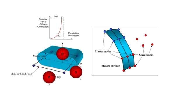
Interface Type 7: Nodes to Surface Contact

1. Automatic node to surface contact interface using the penalty method with variable stiffness
2. A gap is defined around the master segment and the slave nodes
3. The contact gap can be constant or variable
4. Resistive forces are applied to keep slave nodes out of the contact gap
5. The interface time step is computed to insure stability
6. Interface type 7 is a general-purpose interface and can simulate all types of impact between a set of nodes and a master surface. Contrary to interface types 3 and 5, interface type 7 is non-oriented and slave nodes can belong to the master surface. Therefore, this interface can simulate auto-impact, especially buckling during a highspeed crash. Interface type 7 solves all problems and limitations encountered with interface types 3 and 5. The search for the closest segment is done via a direct search algorithm; therefore, there are no search limitations and all possible contacts are found. The energy jumps induced by a node impacting from the shell edges are removed by the cylindrical gap around the edges.

IMPORTANT INTERFACE PARAMETERS:

Tap - Determines how the size of the gap is calculated.

Gap_min - Minimum gap for activation of the interface.

Inactiv - Action to take if initial penetration exists.

Istf - Affects how the stiffness of the interface is calculated.

Iform - Friction formulation

St_min - Minimum stiffness to use in the interface.

Idel - What do with slave nodes and master segments if an element fails(deleted) that they are attached to.

• Here the recommended parameters for the type-7 interface and the friction of 0.2 that we entered are shown below,

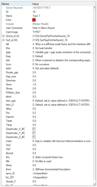
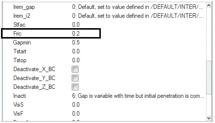
Fig: Selfcontact interface recommended properties

• Now check the penetration and intersection for the whole body of the vehicle by selecting tools>penetration check>select the group in the selection and click check to verify the group whether the penetration occurred or not.
• After checking the penetration it resultant that any occurred or not, hence this group is cleared from the penetration and intersection that is shown below,

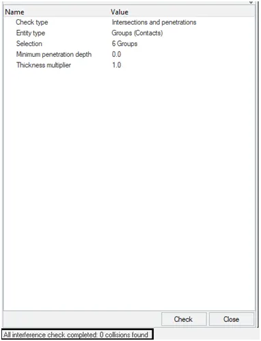
Fig: Penetration Check

• After verifying the penetration and intersection we want to check the rigid bodies by using the model checker option and if any issues may appear then clear that errors. In this model, there are no issues occur.

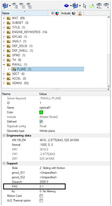
Fig: Rigid body

• Then create a rigid wall to crash the vehicle in a rigid plane(Crash Simulation) and observe the simulation and energy between the wall and vehicle. Right-click the solver>create>RWALL>select plane>enter the properties of a rigid wall of friction as 0.1 and the Dsearch as 2000. Select the engineering data and ensure the axis of XM, YM, ZM which denotes the vehicle movement from normal to a rigid wall. In XM axis we are selecting the vehicle bumper portion
• And in normal N we initiate the distance between the rigid wall and the vehicle bumper.
• Therefore the RWALL properties and the data's given in this simulation are shown below,

Fig: Rigid wall properties

• A created rigid wall of friction as 0.1 and the frontal area is shown as below,
• 

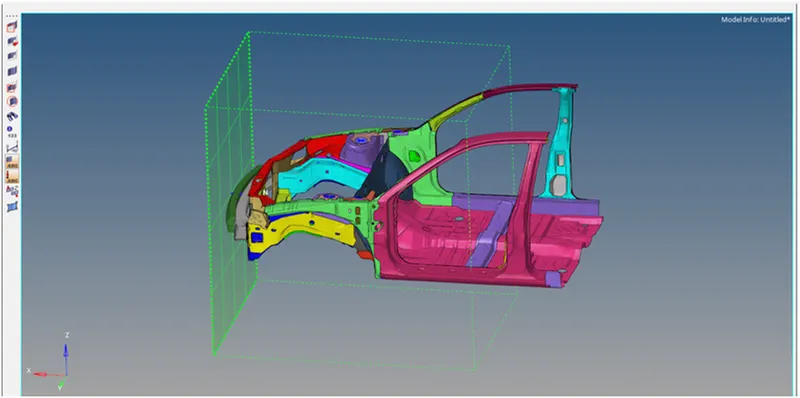
Fig: Frontal car with rigid wall

• Now we want to move the CG in the required range by adding the mass for each node and creating the excess mass for certain selected nodes that is depends upon the movement of CG.
• Ensure that CG should be present between the center of the driver's seat. First, we verify the actual total mass present in nodes by selecting the mass>balancing option in the hyper crash. Before that, import the edited file which is worked on a hyper mesh into the hyper crash.
• Here the actual total mass value shows as 188kg for 300k nodes. To view, the CG click the overview option and view the model it will show the CG as a dot point. That value is shown as below,

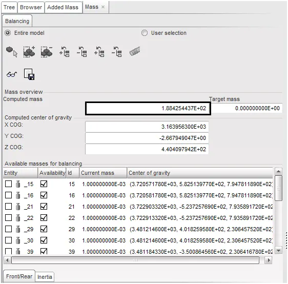
Fig: Default Mass

• To move the CG increase the mass value from 188kg to 700kg that value is mentioned by the instructor. By selecting loadcase>added mass> it shows the total nodes and the mass value for those nodes. Those values and the separation of nodes are set as default. The selection of added mass is shown below,

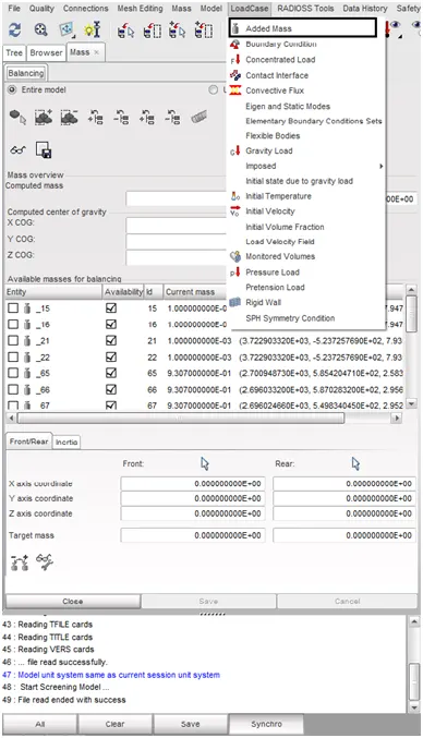
Fig: Added Mass

• In the added mass, click box icon shows 8 different types that depend upon the distribution of mass with group or node. Here select Type=1(mass is distributed to each node of a node group) it will create a section, in that section enter the mass value to add total mass value in the frontal area of a vehicle.
• Balancing the mass value and creation of mass section will move the CG at the required point. The type selection of added mass is shown below,

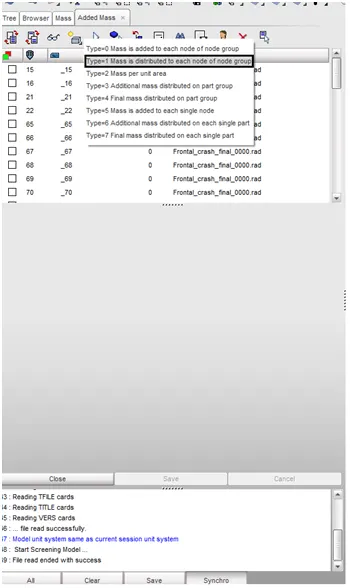
Fig: Mass type

• Therefore the mass is added through the mass type and 8 sections are created each section contains some amount of additional mass added in the particular node that is selected by the user. Now added mass section and the selected nodes are shown as below,
• 

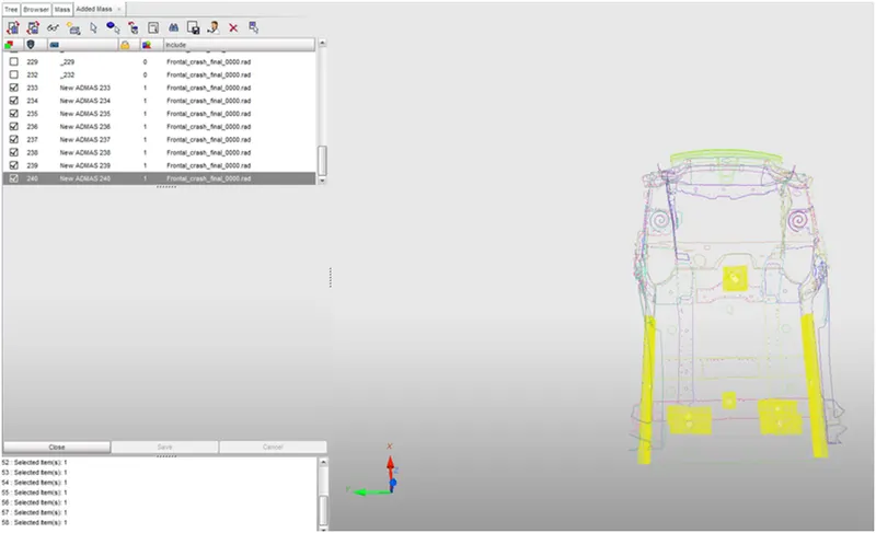
Fig: Section added mass

• Now the total mass is reached as 700kg by adding the new mass value for some specified nodes and that value is initiated below,

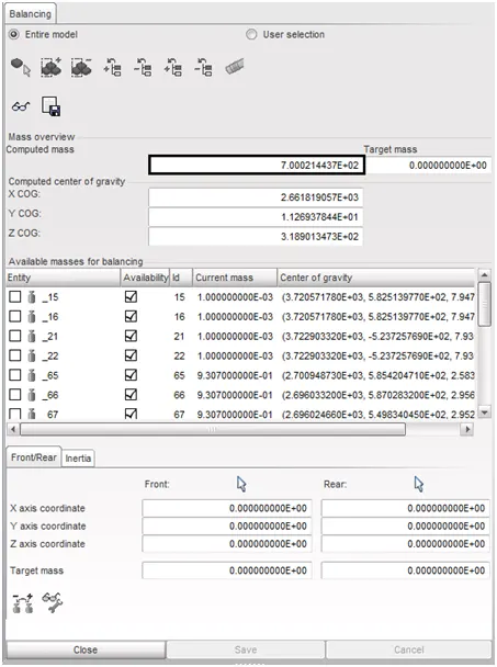
Fig: Value-added mass

• By changing the mass of 700kg the CG has reached a required range that is in between the driver seat and B pillar. Mass balancing is used to change the mass value and to move the CG by adding the mass in different valid nodes. Hence CG is moved and that is shown as below,
• 

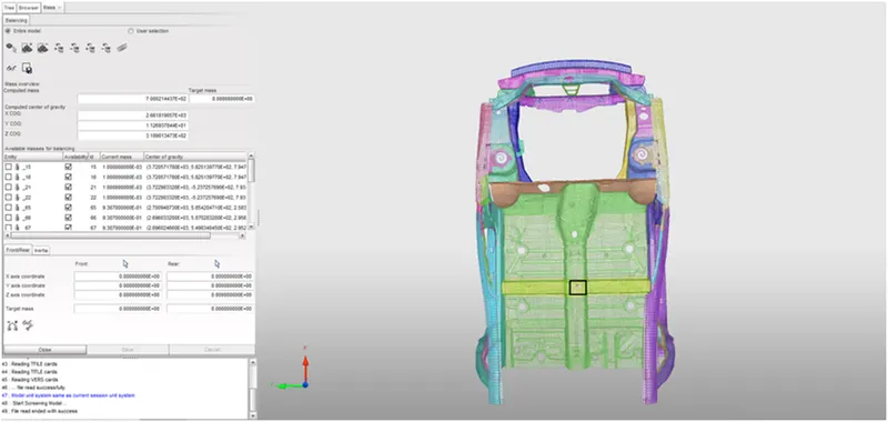
Fig: Centre gravity point

• Now we want to give the initial velocity of a vehicle as 35mph that is given by the instructor. By right-click the solver>create>INIVEL> setup the properties by giving the value of velocity as 15.65mm/ms it is obtained by converting the unit to 35mph. Then click the gmd_ID and select the groups and confirm it.
• Therefore the initial velocity is created and that is shown as below,

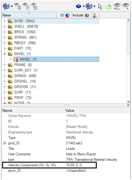
Fig: Initial velocity

• After creating an initial velocity check whether the model is in good condition or not by using the model checker option. Select Tools>model checker>click run icon it will check the total model and show the results. If any errors will appear after the completion of the model checker clear the errors to run the simulation. Here the model checker is run completely and that is shown below,

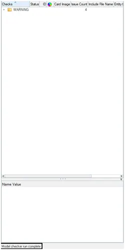
Fig: Model checker

• To mention the time step as 0.5 to 0.1 microseconds by selecting the solver>engine keywords>dt/node and enter the value of Tmin in that setup table as 0.0001. And to set the run time of simulation as 80ms by selecting solver>engine keywords>run>Tstop and enter the simulation run time. The time step and run time setup data are shown below,
• 
• 

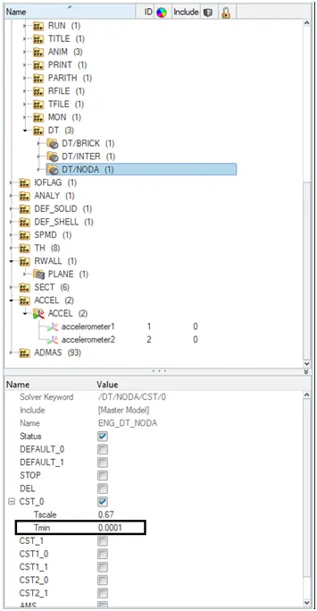
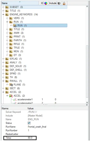
Fig: Timestep and Run time properties

OUTPUT REQUEST:

SECTIONAL FORCE:

• After editing all the setups for simulation then we have to set the output request that depends upon what output we want in that simulation. Here we want to obtain the Sectional force in the rails at the location of indicated node 174247 and parallel opposite side node.
• To create the cross-section by selecting the solver>create>SECT> then we want to create a movable frame in that cross-section and select nodes of origin, X-axis, and XY axis to obtain the normal N direction opposite from the crash direction X. This frame is created to the analysis of F3 force that is normal Z here they are considered as a sectional force while on the crash simulation.
• The below image shows the recommended nodes for sectional force and the created two frames
• 

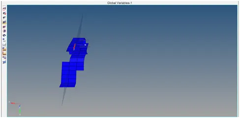
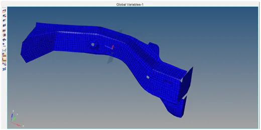
Fig: Cross-section

• We want to initiate the system in section property and to mention the system number in Frame_ID of each recommended section. The cross-section for sectional force in the particular node and the frame id is shown as below,
• 
• 

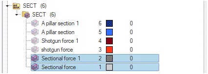
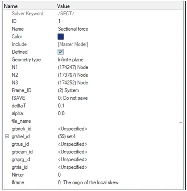
Fig: Cross-section properties

• In a movable frame, we want to select the origin node(N1), axis node(N2), and plane node(N3). The same node intimate in the system is required in the section node ID.
• A node selection and the axis point for the sectional force is shown below,
• 
• 

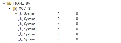
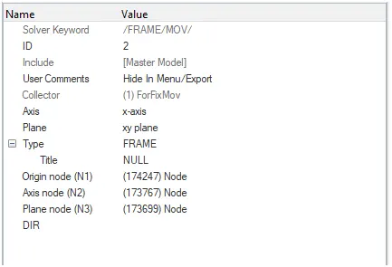
Fig: Frame Properties

AXIAL FORCE:

• Here we want to obtain the output request for axial force received on the rails from the bumper so create the interface group(type-7) for rail and bumper with recommended properties. By selecting the Model>right click and select the create >contact it creates a group and edits the group with the recommended parameters.

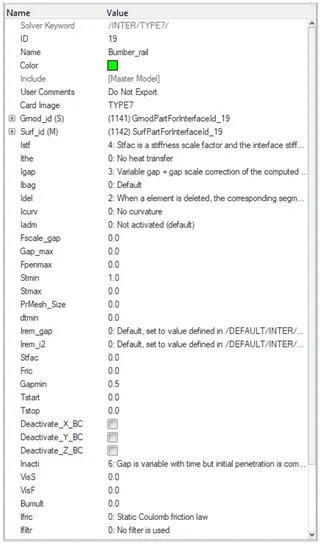
Fig: Interface recommended properties

• Select the master nodes as bumper and the slave nodes as rail and other parameters are mentioned as recommended type-7 parameters. Denote the output block for the Bumper rail group to obtain the axial force received on the rails from the bumper. The master and slave node for this group is shown below,
• 

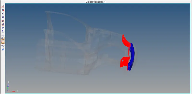
Fig: Master and Slave nodes

SHOTGUN CROSS-SECTIONAL FORCE:

• To create the cross-section by selecting the solver>create>SECT> then we want to create a movable frame in that cross-section and select nodes of origin, X-axis, and XY axis to obtain the normal N direction opposite from the crash direction X. This frame is created to the analysis of F3 force that is normal Z here they are considered as a sectional force while on the crash simulation.
• We want to initiate the system in section property and to mention the system number in Frame_ID of each recommended section.
• In a movable frame, we want to select the origin node(N1), axis node(N2), and plane node(N3). The same node intimate in the system is required in the section node ID.
• The below image shows created shotgun force and frames
• 

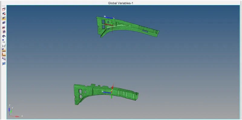
Fig: Shotgun cross-sectional force

A-PILLAR CROSS-SECTIONAL FORCE:

• To create the cross-section by selecting the solver>create>SECT> then we want to create a movable frame in that cross-section and select nodes of origin, X-axis, and XY axis to obtain the normal N direction opposite from the crash direction X. This frame is created to the analysis of F3 force that is normal Z here they are considered as a sectional force while on the crash simulation.
• We want to initiate the system in section property and to mention the system number in Frame_ID of each recommended section.
• In a movable frame, we want to select the origin node(N1), axis node(N2), and plane node(N3). The same node intimate in the system is required in the section node ID.
• The below image shows the created A-pillar cross-sectional force and frames,
• 

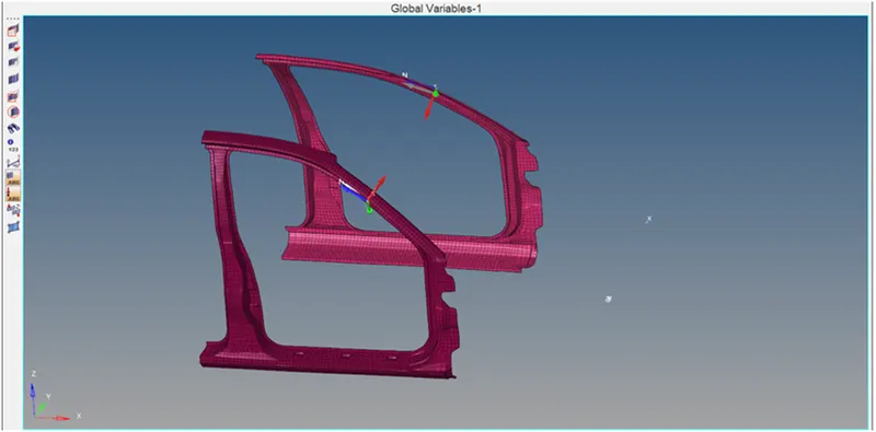
Fig: A-pillar cross-sectional force

• Here all the cross-sections and the frames are shown below,
• 

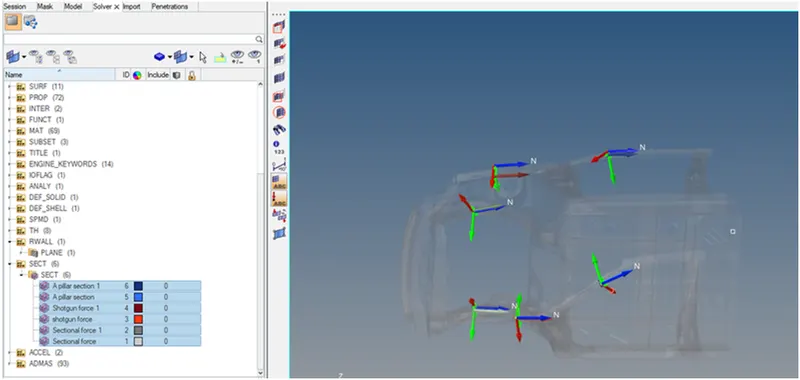
Fig: Cross sections and frames

ACCELEROMETER:

• Here we want to observe the output of the acceleration curve received on the accelerometer at the base of the B pillar. By selecting the solver>right click and select create>ACCEL it will create acceleration now select Entity IDs and pick one node in the base of the B-pillar.
• It creates an accelerometer for that node in B-pillar to analyze the acceleration curve for that node. The same procedure is followed for the opposite node of B-pillar hence it created and that are shown below,
• 

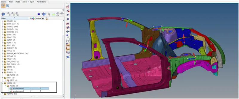
Fig: Accelerometer points

INTRUSIONS:

• To create the Intrusions on the dash wall at nodes 66695 and 66244. By selecting the solver>TH>node> and clicking the select Entity IDs and right-click on the node selection tab and enter the node number it will consider that node for output observation.
• The same procedure is followed for the 66244 nodes hence it is created and that is shown below,
• 
• 

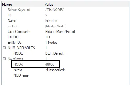
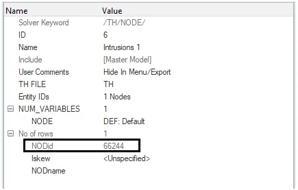
Fig: Intrusion properties

• Intrusions on the dash wall nodes 66695 and 66244 are intimated below,
• 

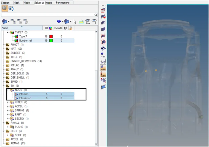
Fig: Intrusion nodes

• Before running the simulation check whether the model is in good condition or not by using the model checker option. Now import the model into the hyper crush and select quality>model checker>click run icon it will check the total model and show the results. If any errors will appear after the completion of the model checker, clear the errors to run the simulation. Here the model checker is run completely and that is shown below,

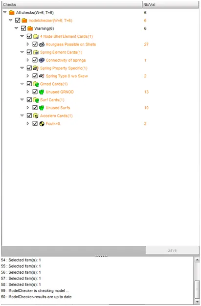
Fig: Model checker

RUN THE ANALYSIS:

Analysis >> Radioss >> Input File: (File Location) >> Hit Radioss

The input file is the same Started file (contains model information) that we had just imported.

The animation video along with the frames will be saved in the same folder where the starter file exists.

Review the Simulation

We have to import the animation file in HyperView first:

HyperView >> FIRST_RUN. h3d >> Apply

1. The tools to review the simulation are available on HyperView.
2. HyperView is a post-processing and visualization environment for FEA that gives the output of the analysis in a simulations format that is user-friendly to understand.
3. From the simulation, we can review how the impact force acts and causes deformations and points of rupture on the model.

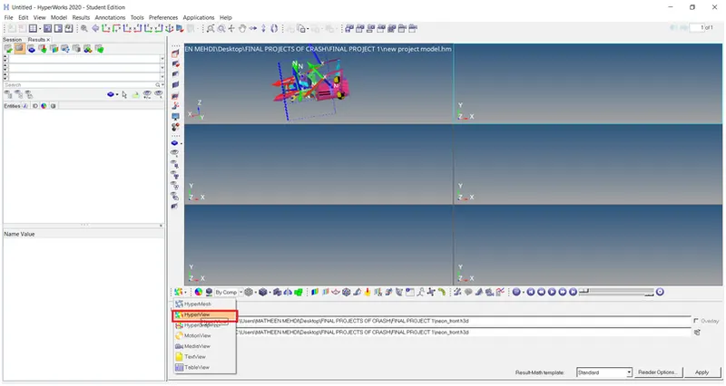
Selecting Hyperveiw

Select Animation file to open

ANIMATION FILE'S

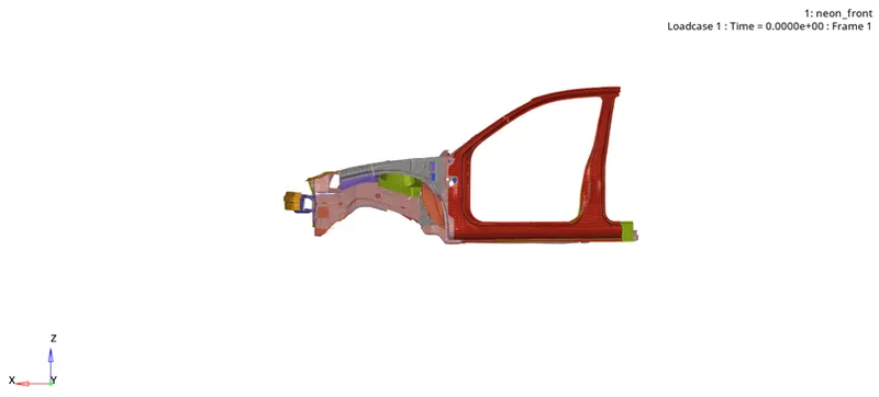
1. Normal View
2. 

2, Von-misses

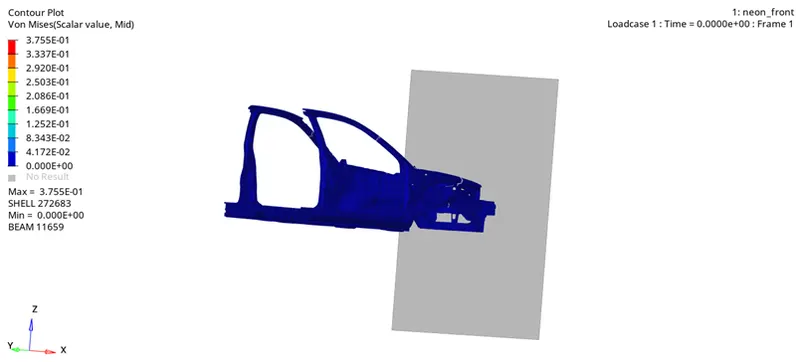
From the simulation, we can see that. Initially, the bumper starts crushing then the bumper forces are transferred to the left and right rail from the rail forces are transferred to A-Pillar LH and RH. In each stage, the forces are going to reduce because energy is absorbed in each stage. Because of no engine blocks, suspension system, etc, the car BIW is going to go down at the end of the simulation

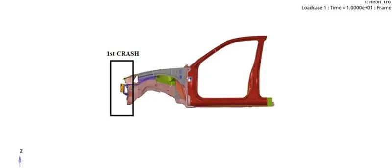
The first bumper starts crashing

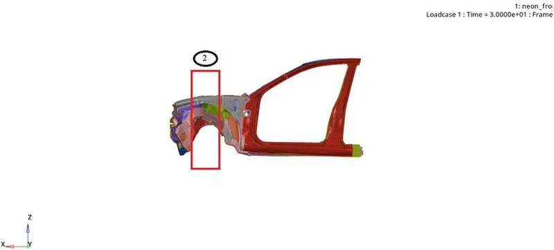
The second Bumper forces are transferred into the rails

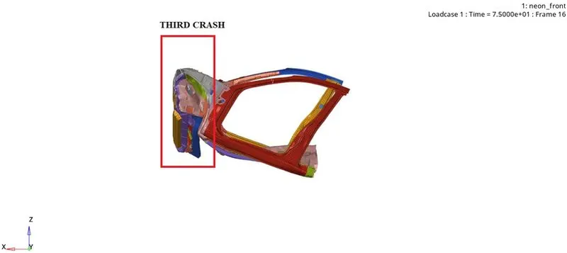
The Third Rails forces are transferred into the A-pillar

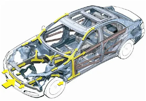
How the forces are transferred is shown in the above figure:

Results after simulation:

1) Energy and Mass error:

• At the end of the simulation, do the energy error and mass error checks and determine whether results would be acceptable
• Open the save location file and click on the output file of the simulation to check for the Energy error and Mass error.
• If the error is negative, it means that some energy has been dissipated.
• In the case of under integrated elements (Belytschko shells, solids with 1 integration point), the Hourglass Energy can explain a negative Energy Error since it is not counted in the energy balance. The normal amount of Hourglass energy is about 10% to 15%.
• If the error is positive, there is an energy creation.
• In the case of using QEPH shell formulation or fully integrated elements, the Energy Error can be slightly positive since there is no Hourglass energy and the computation is much more accurate. An error of 1% or 2% will be acceptable.
• In the case of a larger positive energy, the source of this energy has to be identified. Incompatible kinematic conditions can lead to such a situation.
• If the error reaches ±99%, the computation has diverged; except in the first cycle of a run for which the initial energy of the system was null so that a relatively false energy balance often introduces large relative error.

After simulation run

Check the Starter Output File for Errors:

1. A starter Output file of .out format is generated after analysis.
2. The Output file contains the data during simulation, such as Cycle, Timestep, Energies, and Errors.
3. We have to check for energy and Mass error which means that the solver did not need to add mass onto the nodes to reduce the timestep to further avoid the Hourglass Error.
4. 

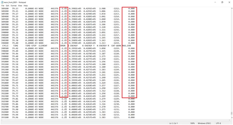
Starter out file

OBSERVATION:

• The Energy Error is Negative and has been linearly increasing up to -2.1% only, which is acceptable.
• Mass error is zero which is acceptable
• We can conclude that there are no errors in the analysis.

PLOT THE GRAPH AND COMPARE RESULTS:

Some basic definitions of energies:

• Energy: Energy, in physics, is the capacity for doing work. It may exist in potential, kinetic, thermal, electrical, chemical, nuclear, or other various forms. In FEA we have Total Energy, Internal Energy, Kinetic energy, Contact energy, and hourglass energy
• Total Energy (TE): Total Energy is the sum of Internal Energy, Kinetic energy & External Work
• Internal Energy (IE): The internal energy of a thermodynamic system is the energy contained within it. It is the energy necessary to create or prepare the system in any given internal state. It does not include the kinetic energy of motion of the system as a whole, nor the potential energy of the system as a whole due to external force fields, including the energy of displacement of the surroundings of the system. It keeps account of the gains and losses of energy of the system that are due to changes in its internal state
• Kinetic energy (KE): In physics, the kinetic energy (KE) of an object is the energy that it possesses due to its motion. It is defined as the work needed to accelerate a body of a given mass from rest to its stated velocity.
• Contact Energy (CE): Contact energy is the energy acting opposite to the system to prevent the penetration acting on the system due to the applied load case.
• Hourglass energy (HE): This is usually done by adding extra stiffness or viscosity across the diagonal which adds extra strain energy into the system and we call this Hourglass Energy.

The tools to plot the graph are available on Hypergraph.

Hypergraph 2D >> Data File >> FIRST_RUNT01 >> Apply

A hypergraph is a data analysis and plotting tool that represents the FEA from the simulation in graphs concerning the selected unit system.

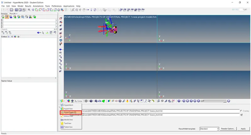
Selecting Hypergraph 2D

Selected T01 File (Time history file)

GLOBAL VARIABLE GRAPHS: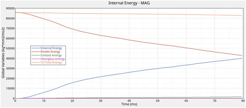

Global variable VS Time

INTERNAL ENERGY AND KINETIC ENERGY:

Internal energy is nothing but the Heat of the System. When the Kinetic Energy is Decreases, the Energy absorbed by the system increases i.e we all know that Energy neither be created nor be destroyed. Once the vehicle is moving with a certain velocity (Say 15.646mm/ms for the Model), the initial kinetic Energy will be High (Refer to Above Graph). Once the car is hit by the rigid wall, the vehicle starts deforming resulting in absorbing the Surrounding Energy and Storing it. Thus, internal Energy starts increasing. At the Maximum deformation, the Velocity will become Zero and thus the kinetics Energy will also be dropping down to zero resulting there is no energy to absorb in the system. Thus, Internal Energy Remains Constant thereafter.

Once after the simulation, The maximum kinetic energy is found at 85708 kN/mm at t=0 and the maximum internal Energy is at 39935.1 kN/mm at t=79.5ms.

CONTACT ENERGY AND HOURGLASS ENERGY:

From the above graph, we can see that the Hourglass energy is almost negligible since we have used Improved integrated element formulation (QEPH).

Ideally, all of KE should be converted into IE and the Total Energy must remain constant, but in our case, since we have Hourglass Energy error, our Total Energy is decreasing. We can rectify this hourglass energy by further reducing the Timestep of the simulation and giving the Ideal Properties wherever we can. Our Requirement from an Ideal Simulation is that we have minimal Contact energy and maximum Energy absorption/Deformation in the elements. We can check the Energy error in the Engine output file, which has maxed out at -2.1% which is within the limits for it to be. Our Mass error is also 0% which means that the solver did not need to add mass onto the nodes to reduce the timestep to further avoid the Hourglass Error.

Contact Energy is nothing but the opposite energy generated from the System to Avoid Penetration. To avoid penetration, we have determined the Gap min value to be 0.5. When the car is moving with a velocity of 35mph and hits the rigid wall, it starts deformation at the bumper section and hence the penetration of the elements occurs, and thus the opposite reaction force is also exerted to avoid the penetration. Hence the contact energy increases gradually from zero. The maximum Contact energy found is 1554.8kN/mm at t=79.5ms.

SECTIONAL FORCES:

1. On RAILS:

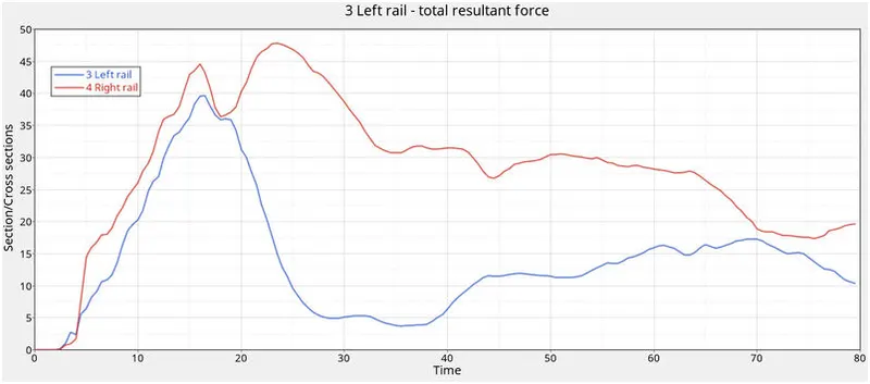
Sectional forces on rails VS time

The maximum cross-sectional force at Left Rail is 39.61 kN/mm at t= 16ms whereas the maximum cross-sectional force at the Right rail is 47.83 kN/mm at t=23.5 ms. The force acting on the rail is the force transmitted by the bumper during the crash. The force transmitted by the bumper to the rail can be unequal due to which the force received at the LH rail may differ from the RH rail. During a crash, the rail will get into direct contact with the rigid wall which will increase the compressive force and then deform. Therefore, the compressive force drops down.

2. On Shotguns:
3. 

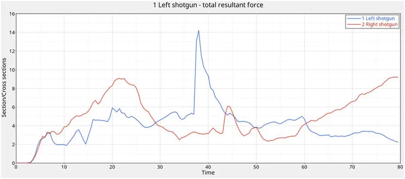
Sectional forces on shotgun VS Time

The maximum cross-sectional force at Left Shotgun is 14.21 kN/mm at t=38 ms whereas the maximum cross-sectional force at Right Shotgun is 9.20 kN/mm at t=80ms. The Force that occurred at the shotgun is the force transmitted from the rail section. The force propagation is not the same at both the rails and hence the amount of deformation at both the shotgun sections are different. Once the Compressive force reaches its maximum value it starts to deform rapidly. Therefore, the Compressive force is decreasing as referred from the graph. As the crash happen continuously, the shotgun will come into contact with the Rigid wall as found in Animation, the rigid wall also exerts the force directly onto the shotguns and hence there is an increase in the Sectional force as seen in the graph.

3. On A-Pillars:

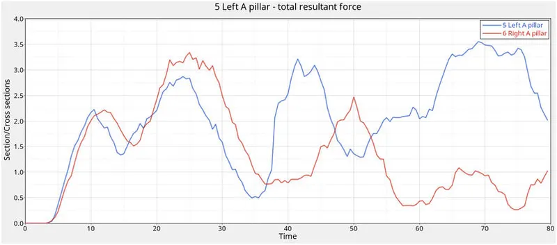
Sectional forces on A-pillar VS Time

The maximum cross-sectional force at Left A-Pillar is 3.5 kN/mm at t= 69 ms whereas the maximum cross-sectional force at Right A-Pillar is 3.33 kN/mm at t=25 when the car hits the rigid wall, there will be some amount of force coming into the A-pillar at both sides. These forces coming to the A-pillar are nothing but the force transmitted from the rail and the shotgun. The force flowing into the LH and RH of the A-pillars will not be equal and hence the deformation of the elements will differ accordingly. During a frontal crash, the sectional force reaching the A-pillars is coming in from the rails and shotgun, hence the force at the A-pillars will be less when compared to the front sections. When the compressive force between the wall and car is maximum, the rail and shotgun get in contact with the rigid wall which causes the shotgun and rail to exert more force. This force then propagates to the A-pillars and hence the force reaching the A-pillar increases again.

INTRUSION SPRINGS:

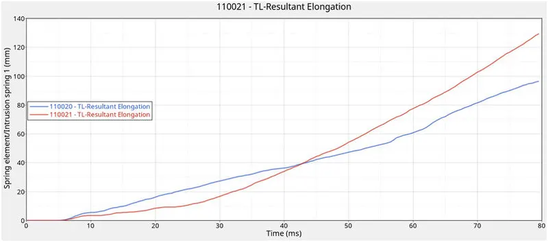
Intrusion spring VS Time

To check the Intrusion at the dash wall at the particularly given node, we have created the spring over the place. The intrusion at this particular node is calculated to check whether the crash will result in the safety of the driver due to the deformation that occurred at the front portion of the vehicle. From the above graph, we can see that the maximum intrusion occurred in the spring (Node 66695,121754) during a crash is 96.56 mm and the maximum intrusion occurred in the spring (Node 66244,121868) during a crash is 129.47 mm. Practically this elongation referred to which extent the foot pedal or the passenger's legs will move once the crash is happening. From the animation, we can notice that there is not much deformation that occurred at this location and the elongation is also low. Hence, we can conclude that there are fewer injuries will happen to the Passenger/driver.

ACCELEROMETER:

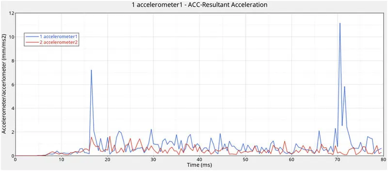
Accelerometer VS Time

As we all know that an Acceleration is the rate of change of velocity. To measure the acceleration, we have placed the accelerometer near the Rocker of B-Pillar on both sides. From the above graph, we can see that initially, the acceleration is constant before the vehicle hits the rigid wall. Once the Car hits the rigid wall with the initial velocity, The acceleration of the vehicle during the crash is not constant across the structure. The front of the vehicle slows down immediately as it hits the rigid wall, while the rest of the structure decelerates at a slower rate as seen in the graph. As seen from the graph there is a sudden increase in the acceleration, this might be because of some vibration that occurs during the crash concerning the point where the accelerometer is placed.

Maximum acceleration at LH = 11.15 mm/ms2 at t=70.5 ms

Maximum acceleration at RH = 1.631 mm/ms2 at t=20.5 ms

AXIAL FORCES ON RAIL OF BUMPER:

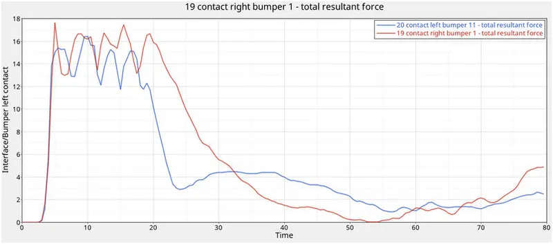
The force from bumper to rail VS Time

From the graph we can see that initially there is no axial force is transmitted from the bumper to the Rail. Once the Vehicle hits the rigid wall, first the Bumper will start deforming transmitting the strain energy to the rail sections. From the graph, we found that the Maximum axial force received from the bumper to the LH rail is 16.41 kN at 10 ms and the Maximum axial force received from the bumper to the RH rail is 17.62 kN at 5 ms.

Learning Outcome

1. Learned how to set up a frontal crash test.
2. Learned how the Rigid wall interface works and can lead to incompatible Kinematic conditions.
3. Learned how Sectional forces are generated.
4. Learned how the distribution of forces among the components during a frontal crash.
5. Learned how some components are designed to deform in such a way to ensure the safety of the passengers inside the cabin.
6. Learned how to check for Energy, mass, and momentum balance.
7. Learned how to Debug errors to get the right results.

CONCLUSION:

The given model was simulated for the frontal crash using Radios and the results obtained were validated. The graphical results were plotted for all the test cases. From the simulation, it can be observed that there was minimum deformation in the cabin, and also minimum intrusion was found in the driver’s seat area