Frontal Crash Simulation following FMVSS 208 guidelines
Aim:
To setup the given simulation conditions on the BIW model for frontal crash simulation in HyperMesh/RADIOSS and discuss about the results obtained.
Procedure.
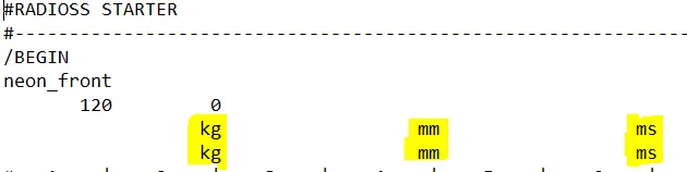
1.check 0000.rad file for the unit sysetm used for the model, for this study Kg, mm, ms unit system will be followed.
2.Import the FE model of car in the hypermesh.
3.set up the model for frontal crash analysis and review the results obtained.
Steps for analysis set up.
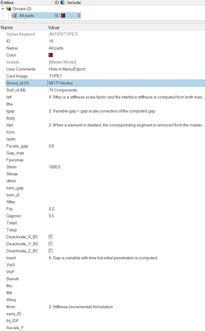
A. Create appropriate interface, friction 0.2 and recommended parameters.
B.check for initial penetrations in the model and solve the initial penetration if any.
C.Rigid wall creation with friction value of 0.1.
D.To apply the mass to the given BIW to reflect the real vehicle mass and to adjust the centre of gravity of the whole model.
E. To apply the initial velocity of 35 mph i.e., 15.6464 mm/ms to the model.
F. To set the elemental and nodal time step to 0.1 – 0.5 microseconds (5e-4 ms) to speed up the simulation.
G. Create the sections in areas where forces need to be calculated.
H. Set up accelerometer on the rocker, bottom of both the B-pillar , to get the acceleration values.
I. Create TH/NODE for selected two nodes on the dash wall area to calculate the intrusion (displacement in x-axis) w,r,t local skew.
setup procedure.
Unit system followed for the model.
A. Interface creation.
Delete the interfaces present in the model, and create a new interface type 7, and select all the parts as master and slave, set the appropriate parameters for the interface as shown below.
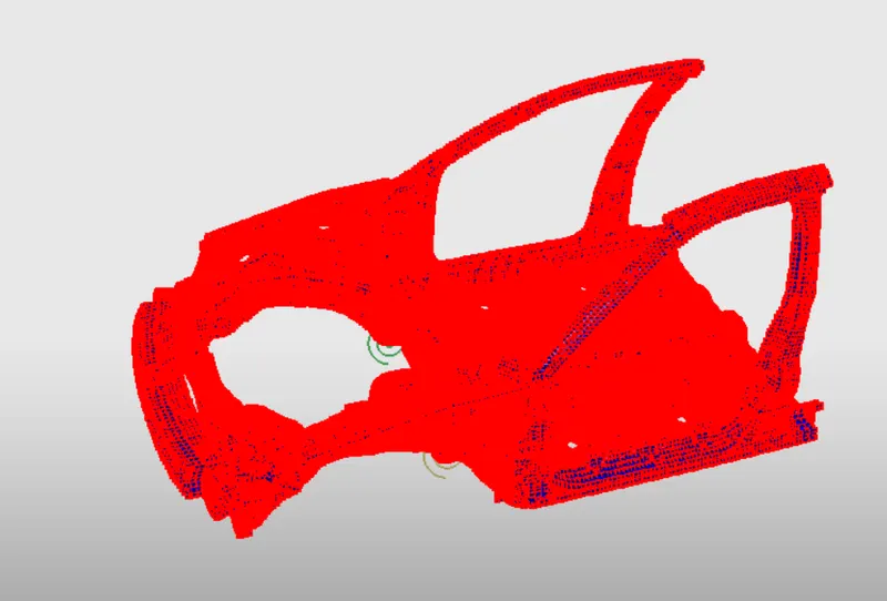
Select all the parts and nodes for slave and the master segments.
B. Initial Penetration check.
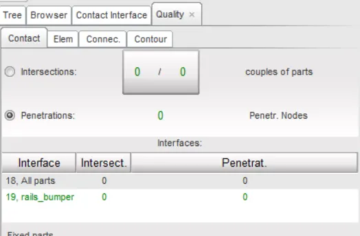
the created interfaces have no initial penetration in the model.
C. Rigid wall creation.
Creat -> Rwall -> Plane.
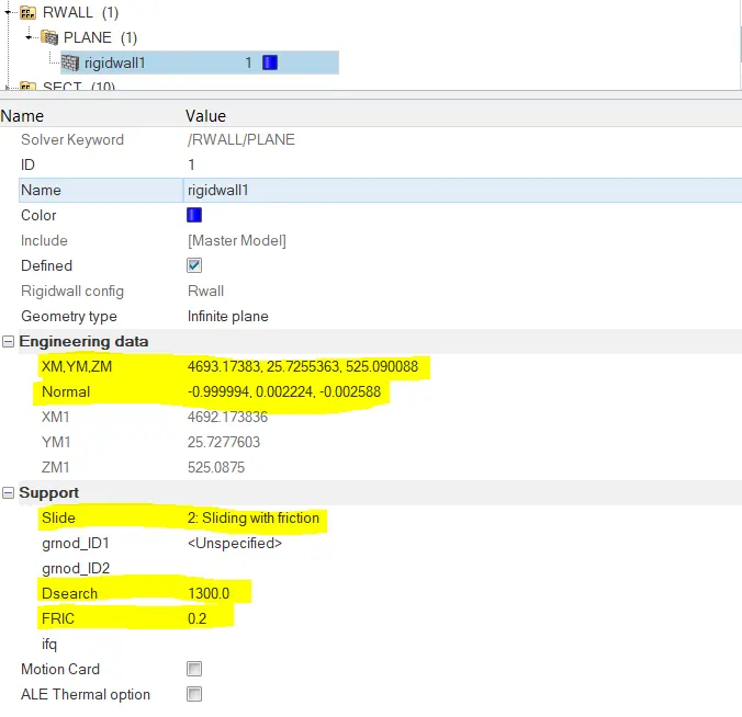
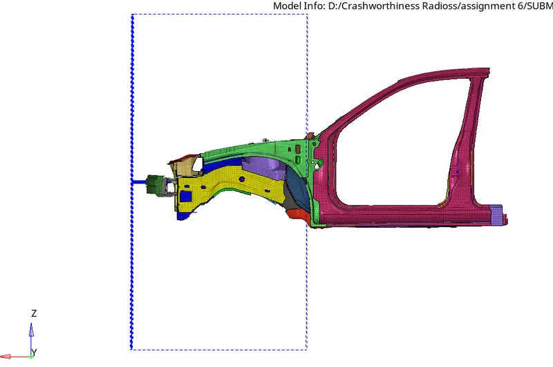
select the base node of the rigidwall and normal vector co-ordinates, select sliding with friction and apply the search distance and friction value to it as shown below.
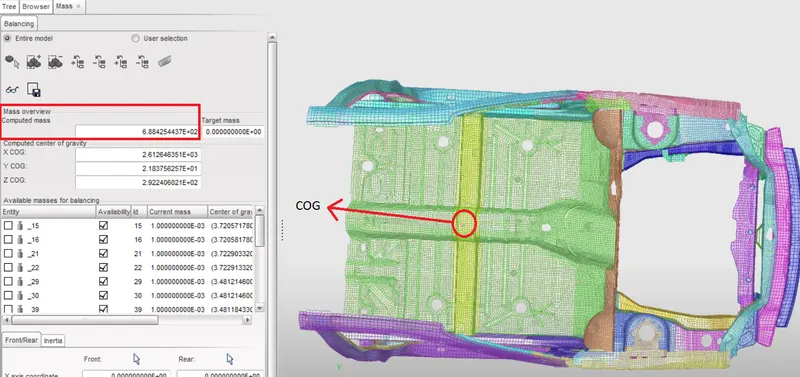
D. To check the COG o fthe model.
Check the model for COG and add the missing masses of the components to th emodel to bring the COG of model close to the COG of full scale model.
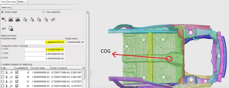
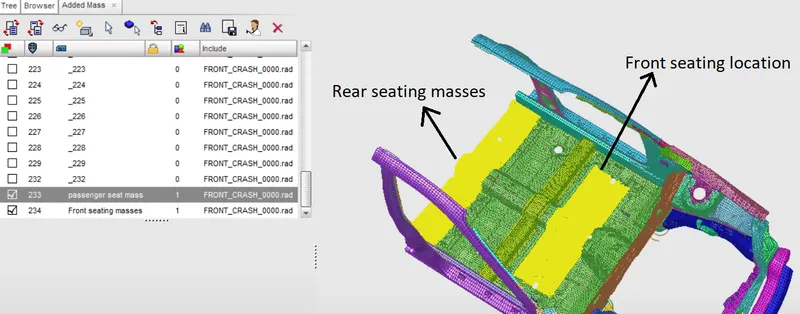
To place the COG of the model to the appropriate place, add the missing masses in the model, for the given model, added masses are the front seating masses which include driver seat and front passenger seat mass, rear seating mass and the tank masses of the vehicle are added.
COG location of the final model, and the final mass of the vehicle is 688.425Kg.
E. Applying the initial velocity.
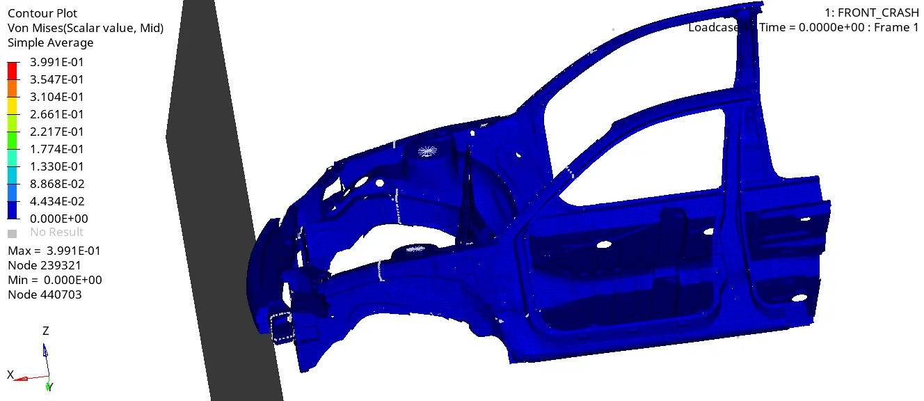
The initial velocity of 35mph i.e., 15.6464 mm/ms is applied to the model by selecting all the nodes.
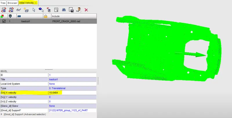
The image above shows the applied initial velocity is in positive X direction.
F. Applying the minimu nodal time step for the simulation.
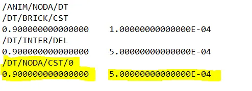
Nodal time step between 01 to 0.5 microseconds (0.5e-3 milliseconds) is applied to the simulation
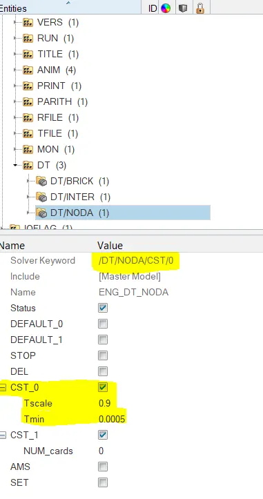
scale factor of 0.9 and minimum nodal timestep of 5e-4 millisecond is applied to the simulation, this printed in the 0001.out file as shown below.
G. Section crestion for calculation of forces.
To creat a section in a desired place, select the N1, N2, N3 nodes normal to the direction of the section and select the group of nodes nad elements to creat the section.
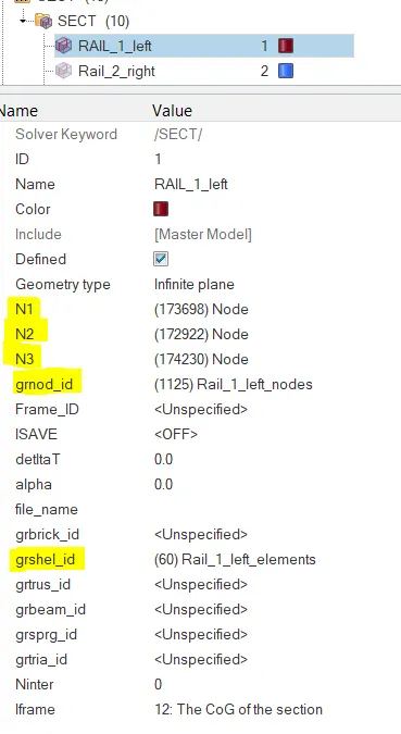
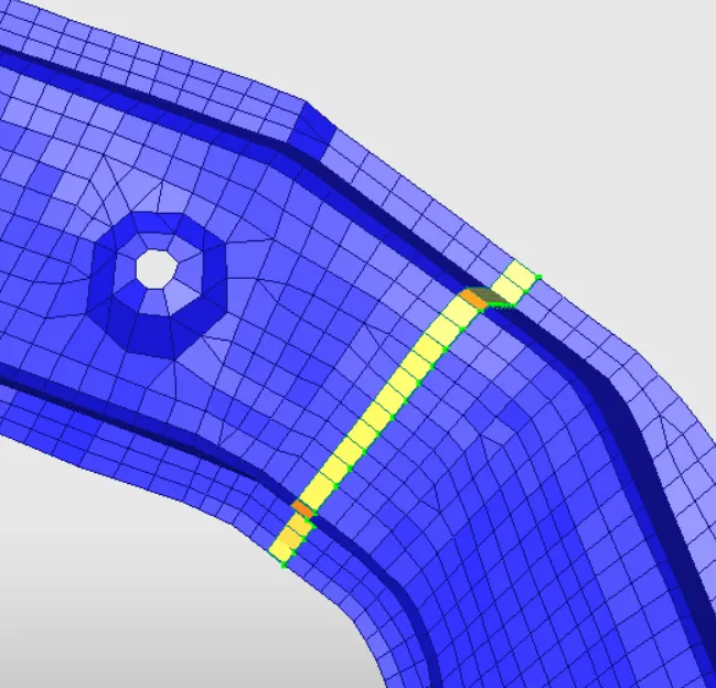
Repeat the steps on the parts where the section creation is required.
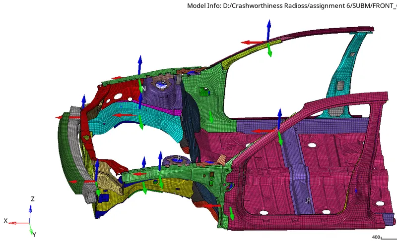
H. Accelerometer for acceleration calculation on the rocker.
Select the Node where the accelerometer is required and define the function value.
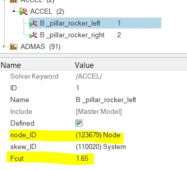
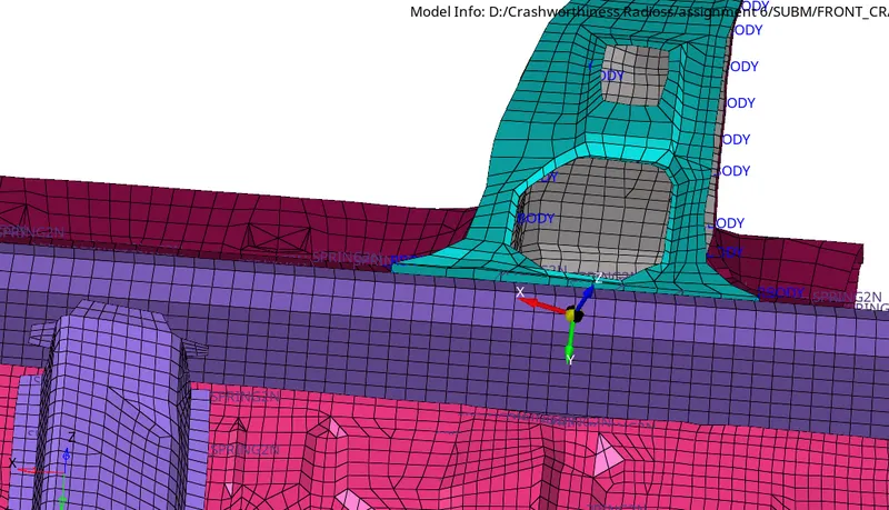
repeat the steps on the other side of the model.
I. intrusion calculation on the dash board.
to calculate the displacement along X direction, Time history of nodes w.r.t local co-ordinate system is requested in the model.
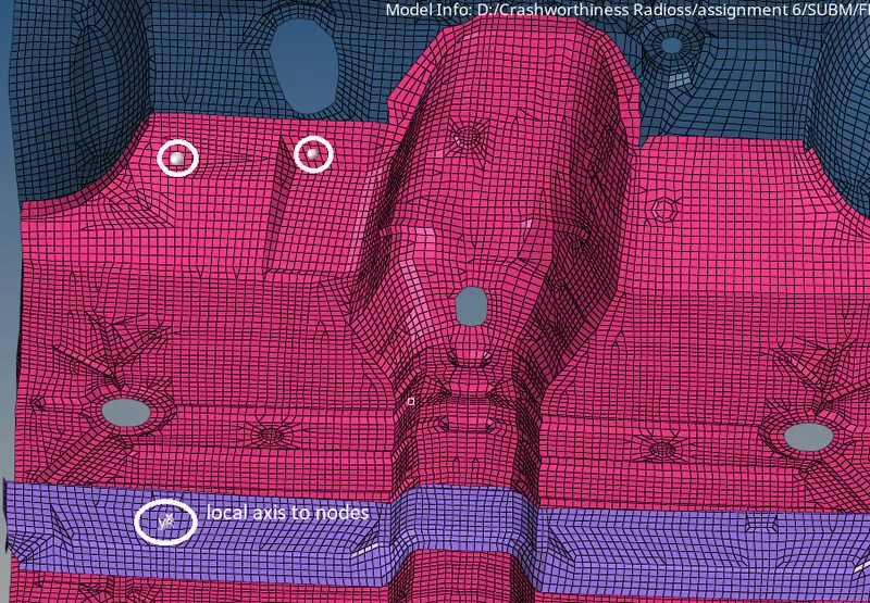
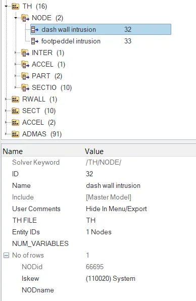
Check the model for any error using model checker, and fix any error which might effect the simulation.
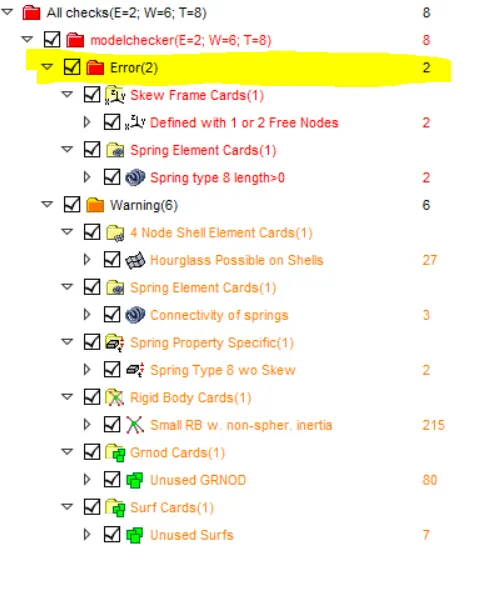
for the model their are 2 error messages, bothe error have no effect on the reusults requested or does not effect the simulation run, delet the elements and run the simulation.
Results.
Time for the run and number of cycles cycle.
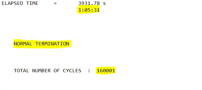
the simulation took 1hr 5min 31sec for completion and normal termination message is shown which indicates the simulation was successful.
ENERGY Error and Mass Error.
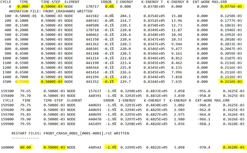
From the image, at Time T=0 the time step is 0.500e-3 which the applied time step for the simulation, and to maintain that time step the propotion of initial mass of 0.977e-5 was added, which is 0.0009% which is less than 1%.
the initial energy error is at 0.0%.
at the end of simulation the energy error is at -1.9% which shows some energy has been dissipiated during the simulation, but it is within the recommended value for energy error i.e., less than 15%.
the final mass error is at 0.03% which is less than 1%, hence the simulation results are wwitin the recommended values.
Hourglass energy in the model.
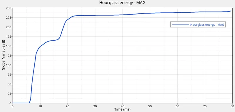
The negative energy error can be explained by the hourglass energy in the model due to reduced number of integration points used in the model for thickness i.e., N which is set to 0 in the /PROP/Shell/
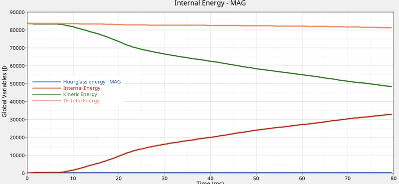
it is observed that the kinetic energy is transefered to internal energy, hence the internal energy increases with time. The total energy of the simulation slightly decreases due to hourglass energy in the simulation.
Forces on bumper.
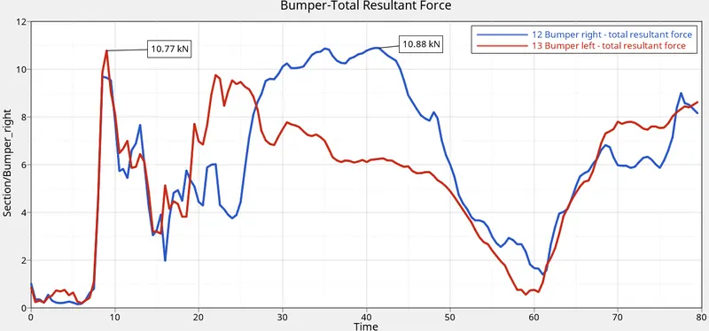
the maximum forces at the location of bumper and rail connection are at 10.77 kN in left side connection and 10.88 kN at right side connection of bumper to rail.
Forces in Headlight Bracket section.
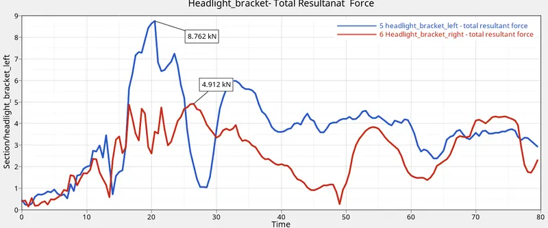
The peak value of force in left bracket is at 8.762 kN where as in Right bracket is at 4.912 kN.
Rail Section forces.
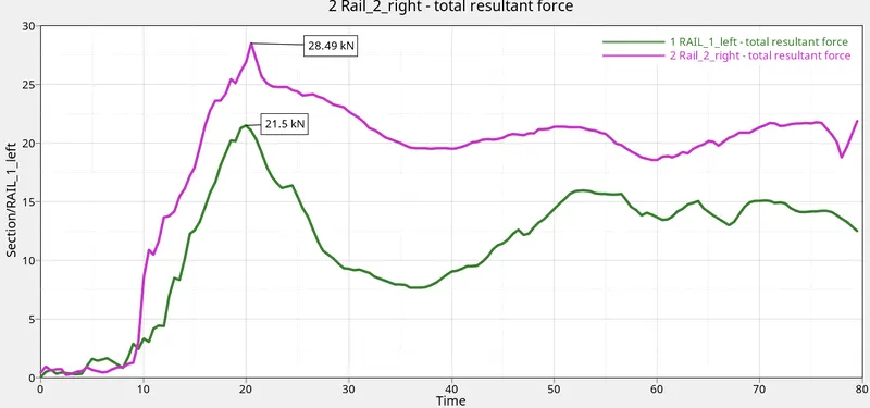
from the graph above it can be observed that the right rail of the model absorbs more forces compare to the left rail, the right rail has a peak value of 28.49kN where as the left rail has apeak value at 21.5 kN forces being transfered to them.
Forces in Shotgun.
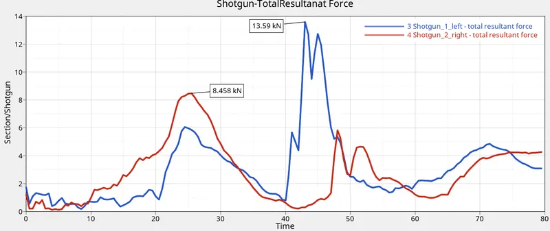
the peak forces are observed in left shotgun section which is at 13.59 kN where as forces in right shotgun is at 8.45 kN.
The observed trend in the shotgun is opposite to the forces obaserved in Rail section, where, right rail had higher peak compared to the left rail.
A-Pillar forces.
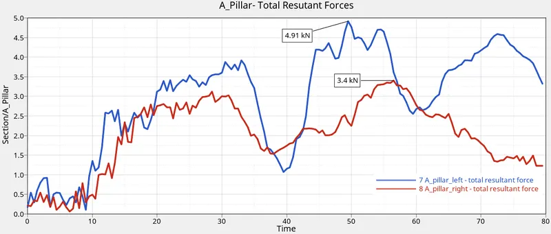
From the graph above it is seen that the forces in Left A-Pillar are higher compared to the forces in right A-Pillar, the peak force in left A-Pillar is at 4.91 kN and that of right A-Pillar is at 3.4 kN.
A-Pillar has most of the connection with shotgun, due to which, the forces from shotgun are transferd to the A-Pillar, hence the left A-Pillar peak is higher than the right A-Pillar simillar to that forces observed in shotgun section.
Acceleration curve.
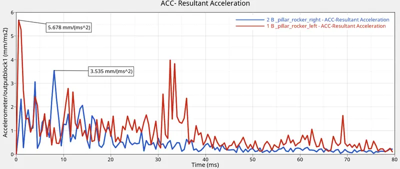
the acceleration curves in the graph show that the acceleration on the left rocker has highest peak at 5.678 mm/(ms^s) compared to that of left rocker which is at 3.535 mm/(ms^2).
Intrusions on the dashwall and footpedal.
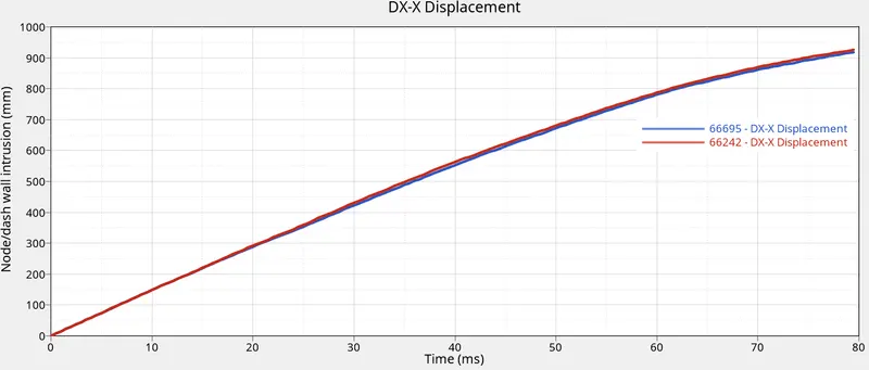
the displacement of bothe the nodes are almost similar to eachother, the displacement in X-Direction is calculated w.r.t local skew defined in the model.
Conclusion.
The given BIW model was set up for fronatl crah analysis, section were created in the impotant areas to calculate the forces and appropriate parameters are requested for post processing to analyse in hypergraph and hyperview.