Frontal Crash of a reduced Chrysler Neon BIW substrate against a rigid wall at 35mph

Objective:- To perform frontal crash analysis of a BIW substrate against a rigid wall at 35mph.

Following steps are followed:-

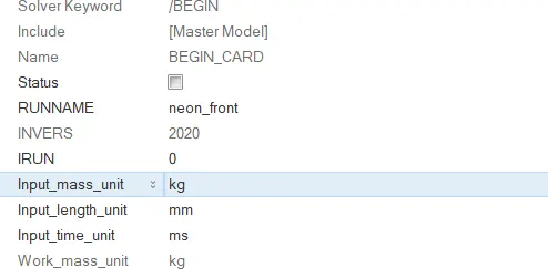
• Check the unit system and either follow[Mg mm s] or [Kg mm ms].
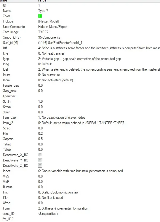
• Create an appropriate interface, friction 0.2, and recommended parameters.
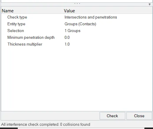
• Make sure of no penetrations and intersection.
• Correct rigid bodies if any issues.
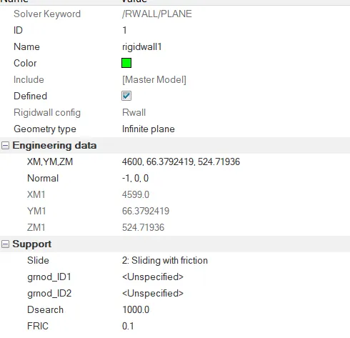
• Create a rigid wall with friction 0.1.
• Compare the model weight with the full-scale 300k nodes model and use added masses to reach target weight 700kg while getting CG about the required range.
• Initial velocity 35 mph.
• Use model checker to ensure good quality.
• Time-step :0.5 to 0.1 microseconds.
• Run 80 ms.

Output requests:

• Sectional force in the rails at the location of indicated node 174247.
• The axial force received on the rails from the bumper.
• Shotgun cross-sectional forces.
• A pillar cross-section.
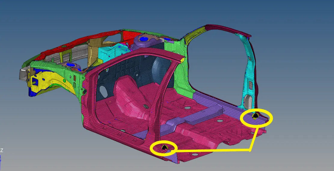
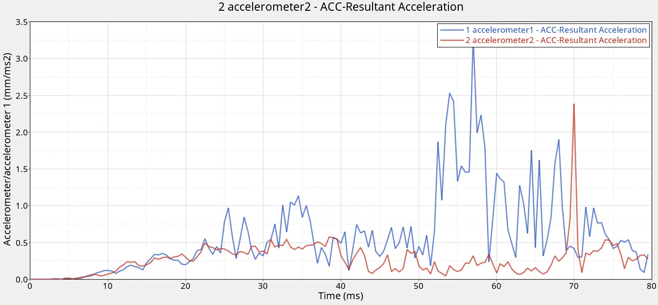
• Acceleration curve received on the accelerometer at base of B pillar (on B pillar rocker).
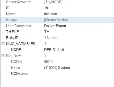
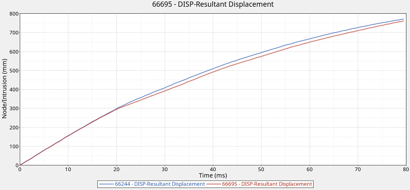
• Intrusions on the dash wall 66695,66244.

• Simulation Set-up:-

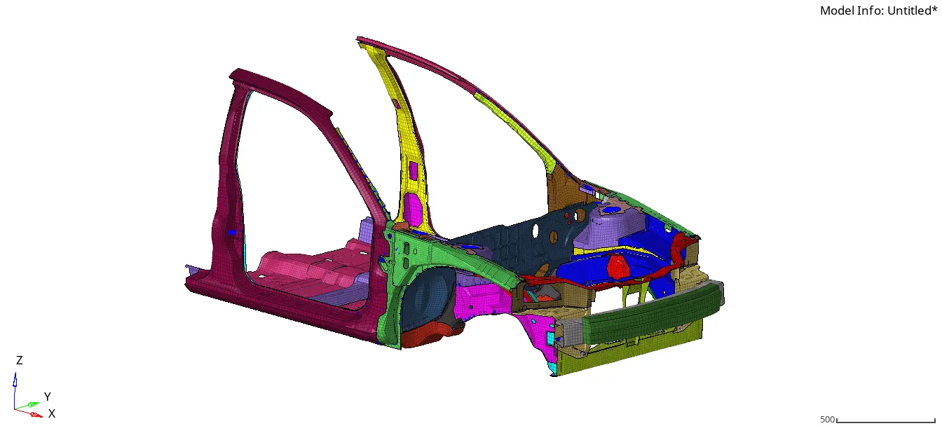
1. Import the BIW substrate solver deck into hypermesh.

2. Check the model units system in the begin card.

3. Create a type 7 self contact interface pertaining to properties mentioned below.

Once the interface is created other interfaces can be deleted.

4. Check penetrations tools

If any penetrations found, they should be fixed because they lead to energy error and also terminations,

Penetrations can be fixed by depenetrate option.

5. Check for rigid body issues Tools

This check will show free parts & free joints. These parts/joints should be fixed else will run into solver issues.

These joints can be fixed by deleting them.=, if any parts are free then they can be fixed by joining them with 1D elements such as springs.

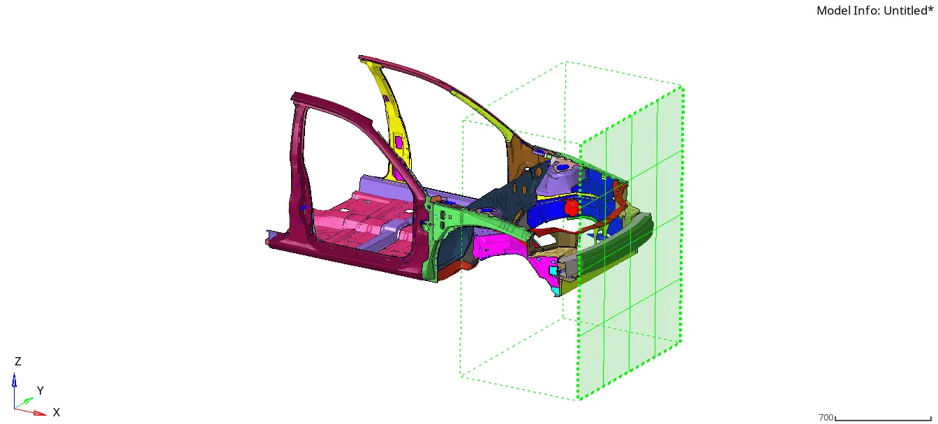
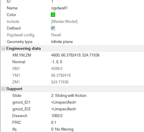
6. Create a planar rigid wall with 0.1 friction. While creating the rigid wall make sure the wall doesn't penetrate with the model, maintain an appropriate distance.

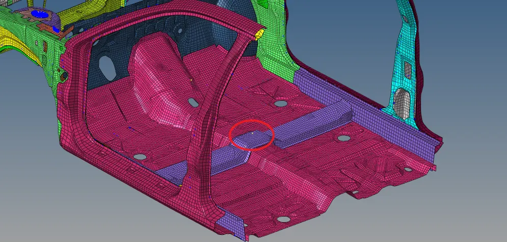
7. Adjust the COG on the cross rail, this can be done using ADMAS, select a node such that the resultant COG will be on cross rail.

A mass of 700kg is added on a node to manipulate the COG near the cross rail. Select the mass as type 0 (mass added to each node of the node group).

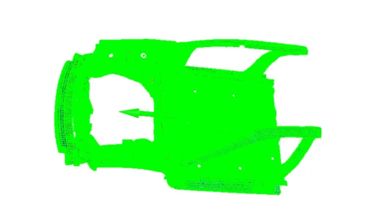
8. Apply the initial velocity of 15.64 mm/ms in the x-direction, initial velocity can be applied by creating the INIVEL card.

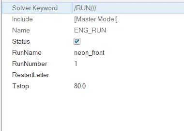
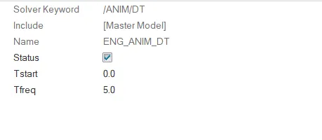
9.Set the time step to 0.5 seconds and the run time to 80 seconds. his can be set in ENG_ANIM_DT & ENG_RUN cards.

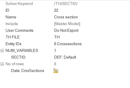
10.Create sections at the right headlight bracket, right A-pillar, right bumper rail, shotgun, and similar sections on the left side.

Sections can be created in the solver tab by first specifying the local coordinate system and then selecting the nodes and elements where we wish to create sections.

Once the cross-sections are created, create an output request card and link these cross-sections so that we can plot the sectional forces.

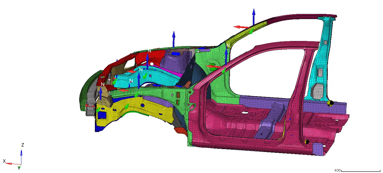
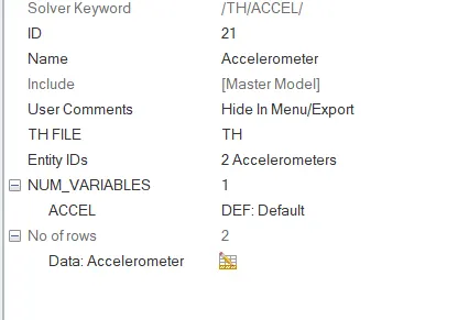
11. Create accelerometers on the B-Pillars and create an output request card in the output blocks by linking these accelerometers to the output block.

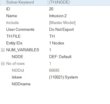
12.Create intrusions on the nodes 66695,66244 so that relative displacement can be measured after crash.

For creating intrusions we need to first create skews exactly parallel to the given nodes and then link them to the output block.

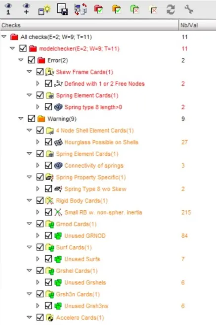
13. Run the model checker (Tools).Few errors and warnings were found out , the errors were fixed and the warnings were suppressed.

14. The model setup is complete, run the simulation. Open the 0001.out file and check the mass and energy errors.

15.For animations open the H3D file in hyper view and for energy plots open the T01 file in hypergraph 2D.

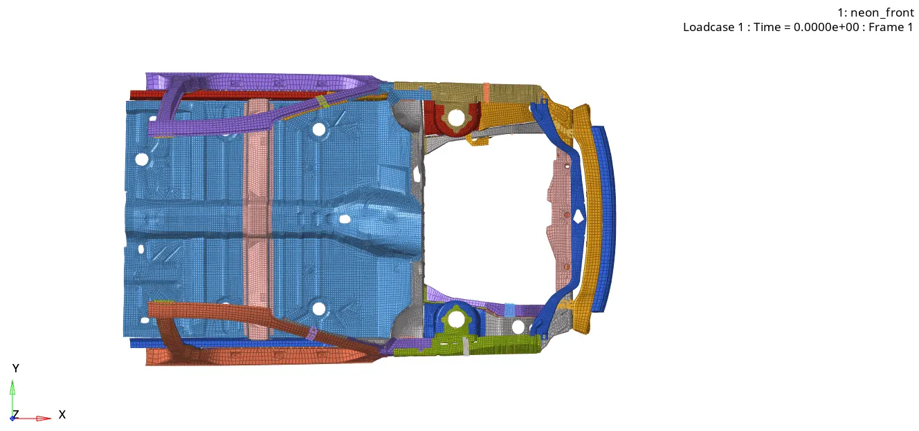
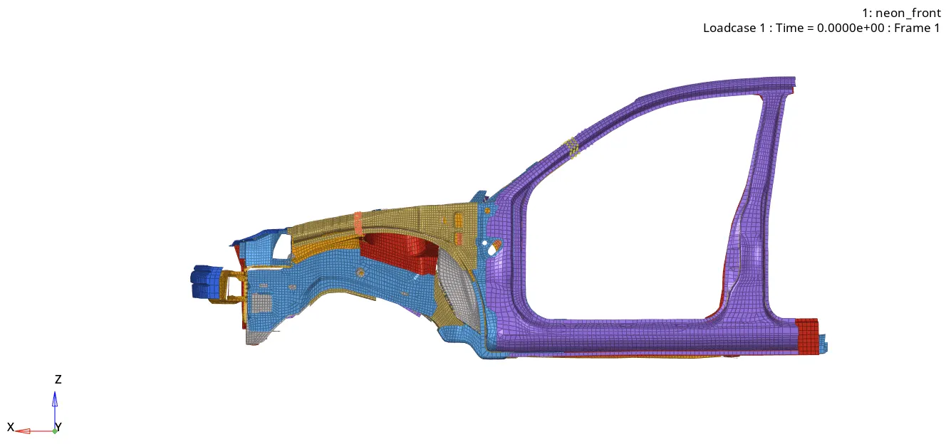
16. Apply von-misses contour to the model with simple averaging.

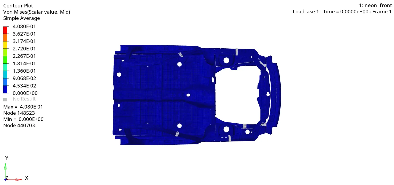
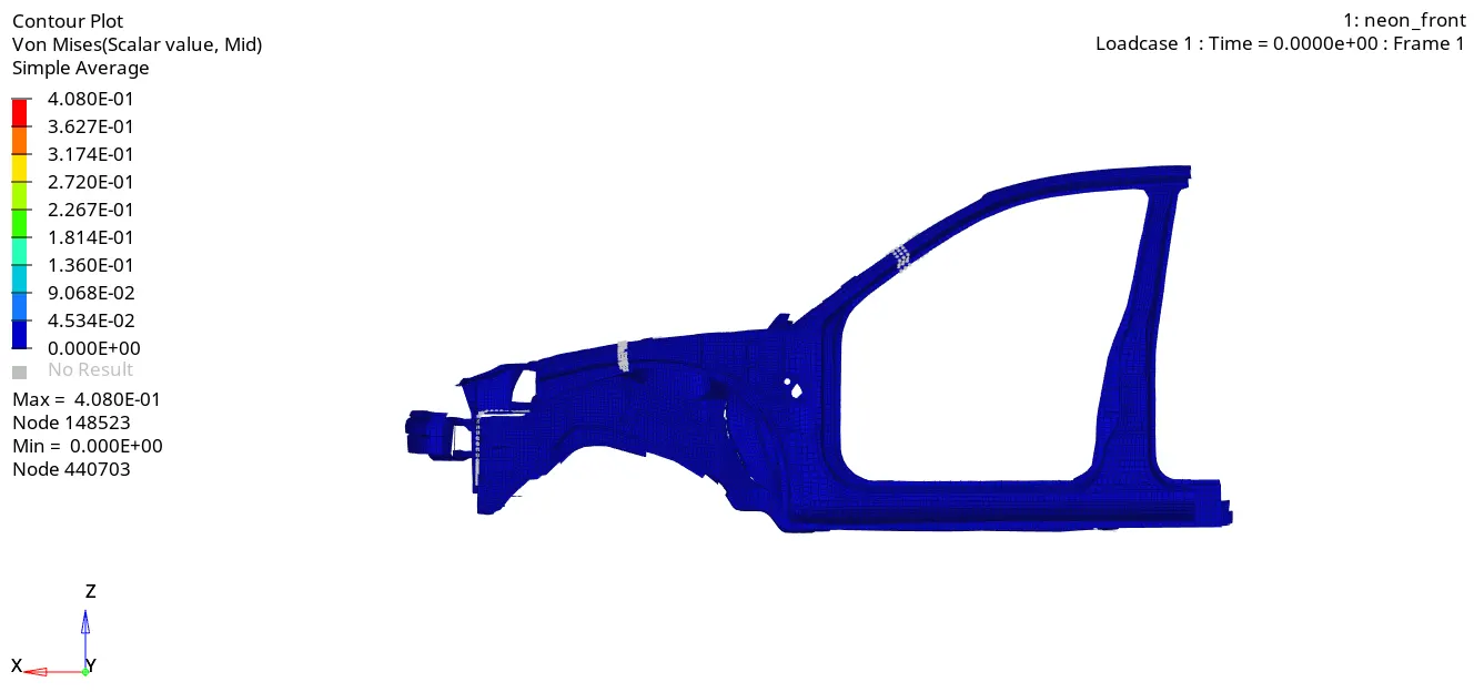
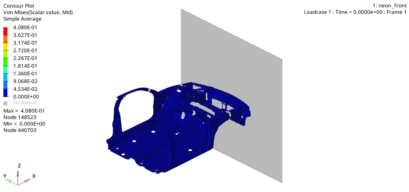
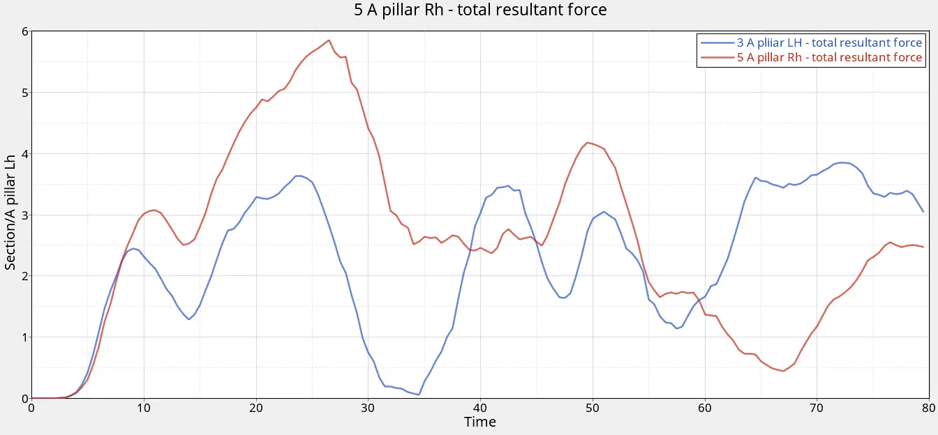
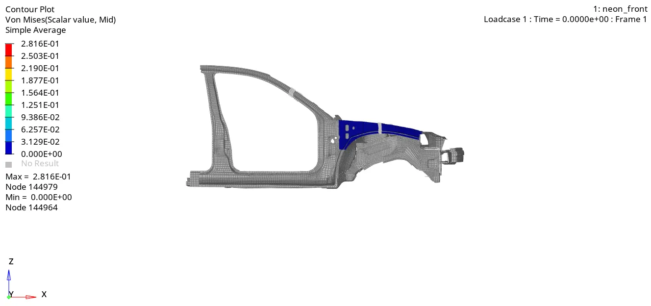
17. Sectional forces at A-Pillar

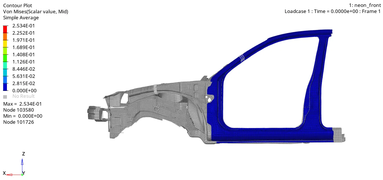
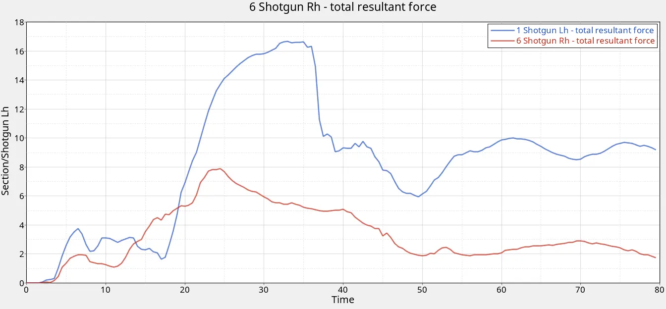
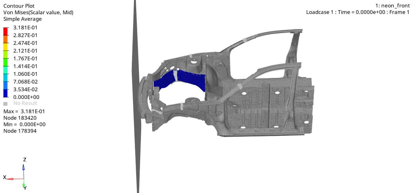
18.Sectional forces at shotgun.

19.Sectional forces at the bumper rails.

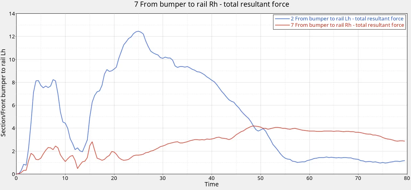
20.Sectional forces at headlight bracket.

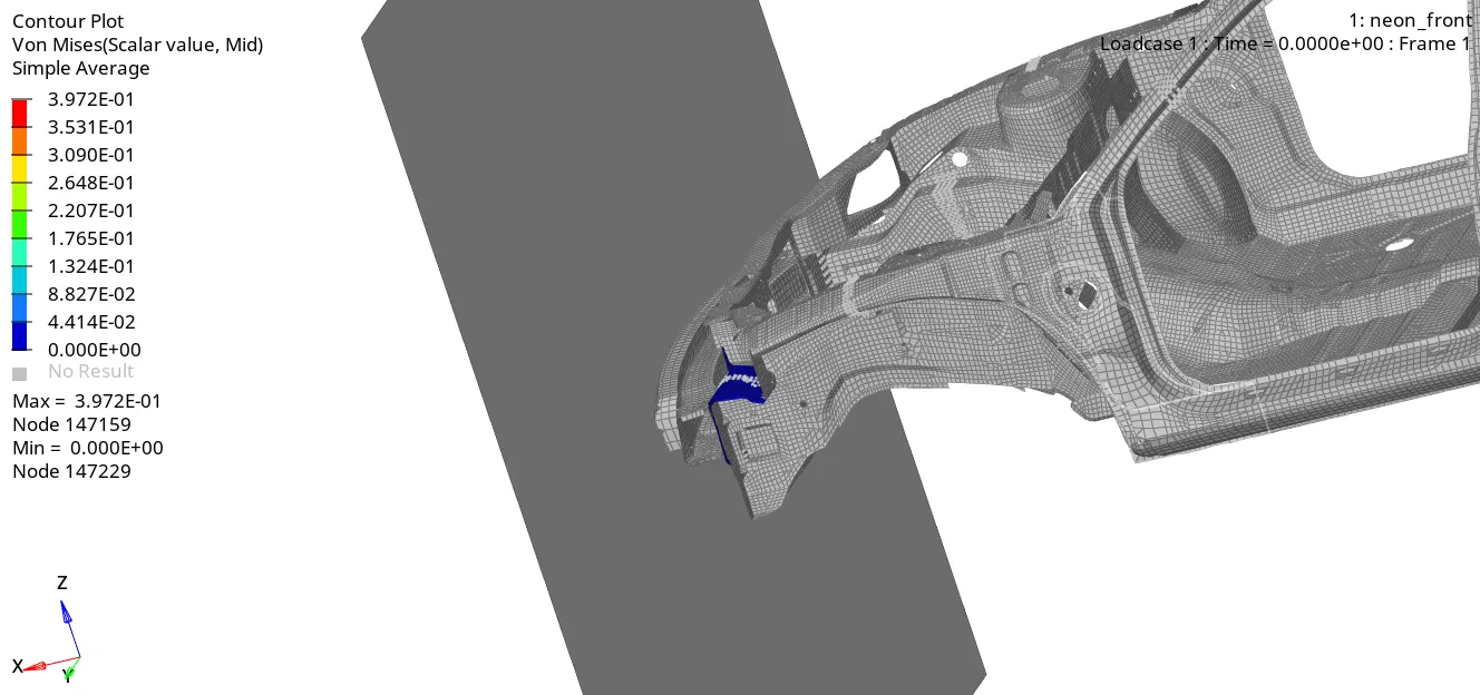
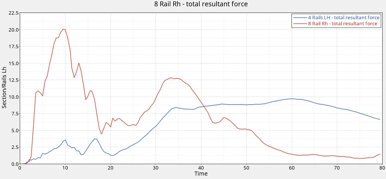
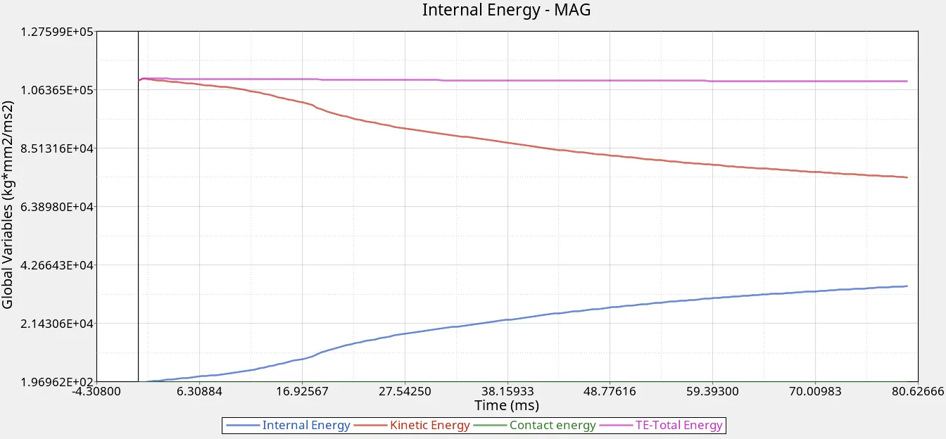
21.Energy plots:- Internal energy, total energy, contact energy, and kinetic energy are plotted.

22.Accelerometer Plots:- The outputs from the accelerometers are plotted.

23:- Intrusion DIsplacement Plots:- The resultant displacement of the instusions of given nodes are plotted.

Conclusion:-

1. The model setup was successful and the simulation was run.

2. The energy error was found out to be -1.6% and the mass error was 0.1271E-02, both are acceptable.

3. Sectional forces were plot along with their contour plots.

4. The deformation on the left side was more as compared to the right side.

5. The relative displacement of the intrusions of given nodes was plotted.

6. Acceleration from the accelerometers was plotted.