Assignment 6

Frontal Crash of Neon

Frontal crash test is one of the major crash test conducted on a vehicle to the check the safety standards. The following project focuses on designing a front crash scenario for the given BIW(body in white) of a dodge neon model and the force distribution across the structure is analyzed.

BIW is basically a joined automobile structure, all the frame components are joined using various joining methods such as rivets, bolts and welds. The name BIW is given due to the fact that the entire component in painted in white. BIW plays a vital role in the crash scenario. It takes up most of the impact load and the keeps the occupants safe and sound. BIW should possess some well defined mechanical features. It should be rigid enough to protect the occupants and it should deform enough to take the impact loading.

For the above reason the BIW basically divided into two parts the crumble region and the frame. Crumble region is which the impact energy is absorbed and it is designed to be crushed. The latter part keeps the passenger’s safety and helps them to walk away out of crash. These two zones are shown below in the picture.

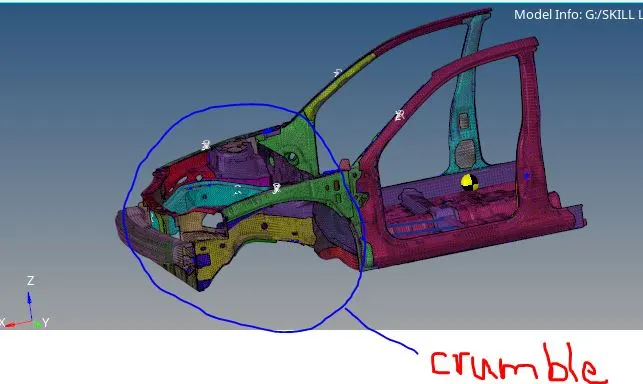
It is so important to design the vehicle which is crash worthy. The simulation of the crash test provides us very essential inputs to the design team to make some important modifications whether to the structure of the material. An accurate simulation of the real time scenario gives an opportunity to the engineer to understand the crash mechanics and design a better product which is crash worthy. Certain parts of the BIW are crucial during the frontal crash. They take significant amount of loads of the remaining structural members. In this project we analyze the force distribution among these components and their behavior during the crash.

1. Case Setup:

Altair Hyperworks is used to simulate the front crash of a neon dodge. Various important parameters such as the contact definition as well as the rigid wall definition and the section creation and the force analysis is done. A detailed description of all the above mentioned is given below.

1.1.Contact

The BIW model is given pre meshed, we will start up with the definition of the contact region. A type 7 contact is used to define the contact, we have few interfaces already defined in the model. These are the subsystem interfaces in the complete model which are not necessary for our model. So they were all deleted and a global interface is created.

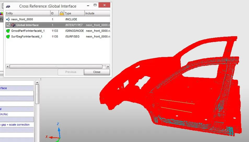
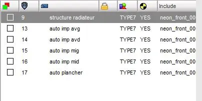
Fig 2: New defined contact Fig 3 : Defined contacts

As we can see from the picture some 6 contacts were defined, for different and they were not properly defined. So to create a global interface we will delete all these contacts and we proceed with a type 7 contact definition. For the slave nodes all the nodes of the BIW are selected and the for the master surface all the elements are selected. The slave as well as the master surface are shown in the pictures below.

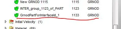
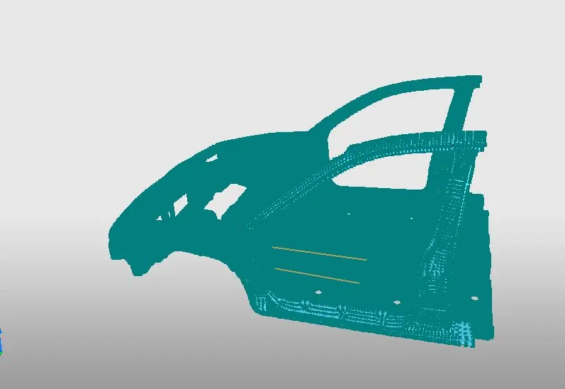
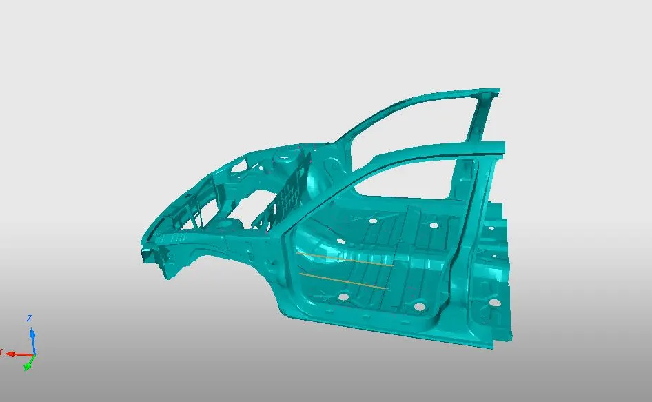
Fig 4: New groupnode Fig 5 : Slavenodes Fig 6 : Master Surface

As per the recommended options for the type 7 contact definition the properties are mentioned in the option palette. All the nodes are formed in to a group and that Grpnod is used as a set in defining slave nodes in the contact.

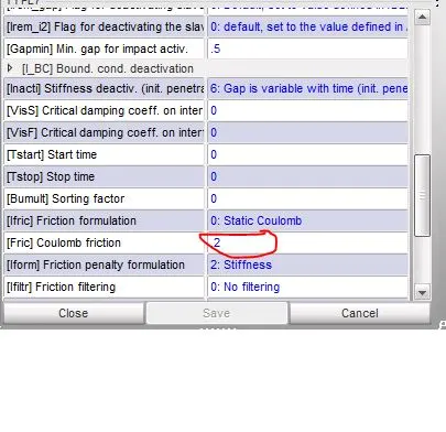
Fig 7 : coloumb friction defined in the cantact type 7

1.2 Units:

It is essential that a consistent system of units is followed throughout the analysis. We can guess the unit system of the model by observing the units of the mass. We have to open the model in hyper crash and then we have to proceed to

mass>balancing

The mass of the components as well as the point masses can be seen in the palette. According to the consistent unit system we can predict the units of the model. We can even see the format of the density. The pictures of the units of the mass and the density are shown below.

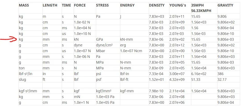
Fig 8 : Consistent system of units, showing the units used in this project.

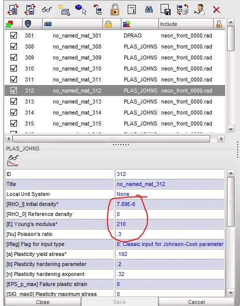
Fig 9 : Units check

1.3 Centre of gravity:

The position of the center of the gravity is very important for an automobile as well as the crash simulation. Initially the COG is close to the dashboard. This is unacceptable as the presence of the mass towards the front will topple the vehicle during the crash. To make the vehicle grounded and stable it is essential to move the COG away from the dashboard.

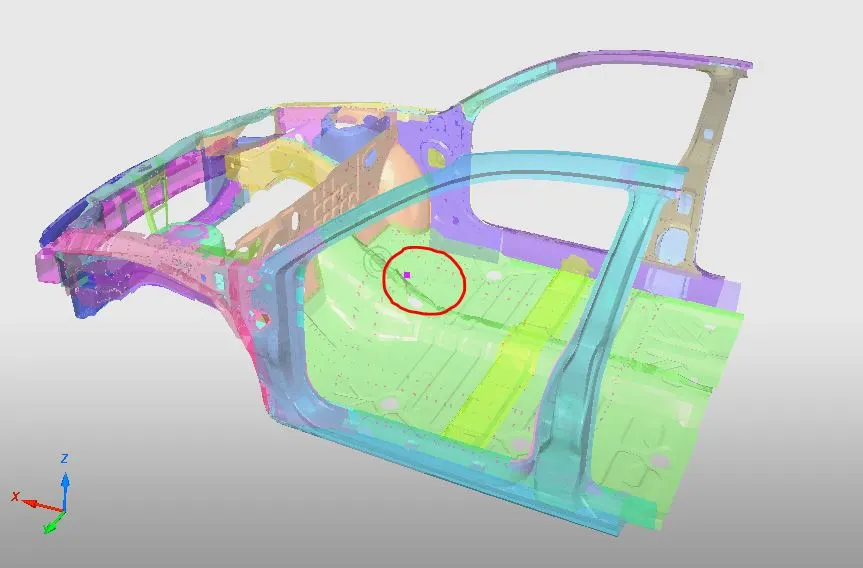
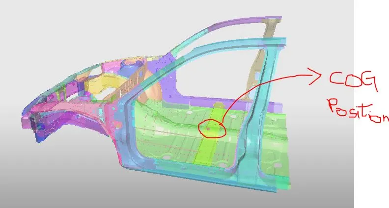
Fig 10: Initial position of COG Fig 11 : New position of COG after adding mass

The mass can be added through the added mass. As we can see from the picture the mass is given as point mass and the value can be changed to add or remove mass.

Suitable mass is added so that the COG is brought back and the overall weight approaches 700 kg. After the addition of the mass at different positions the overall weight reaches 695kg and the COG position is moved to the recommended position.

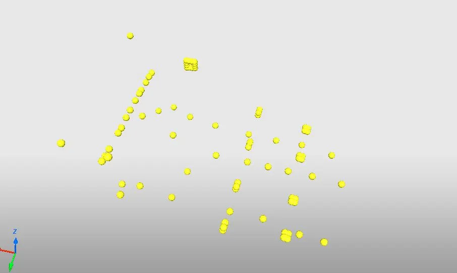
Fig 12 : Mass postions for adding mass

1.4 Free and additional rigid bodies:

As we are dealing with a subsystem there might be few parts which are free and are not properly connected. These can be either connected properly or they can be completely deleted if not necessary. The free parts can be checked using the connectivity of the parts option in the menu bar in hyper crash.

Quality>Check connectivity of tree connection.

The entire model tree is selected and the connectivity is checked using the above mentioned option. We can see tow free parts in the name of spherical joints are free. As there is no specific use for them they can be deleted form the model. The free parts as well as the model is shown in the below image.

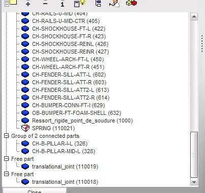
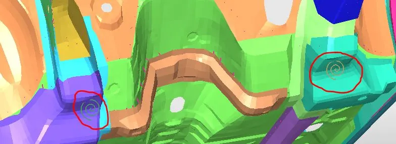
Fig 13 : connectivity check Fig 14 : Spherical joints

Similarly we have to delete the additional rigid bodies. We can find that there are two translational joints at the tree and they are attached to the two skews at the shock absorber housing. The rigid body as well as the skew and the springs connected to them can be deleted.

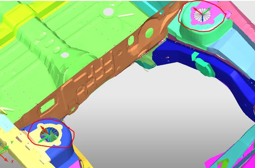
Fig 15 : Extra Rigid bodies and the skews

1.5 Rigid wall :

A rigid wall is created as a barrier for the crash analysis. The rigid wall is created in hyper mesh using the node selection and the normal direction for the wall surface. The Dsearch distance is given 1200 to take account of the entire crumple zone. The wall created at the bumper serves the purpose as a barrier for the front crash.

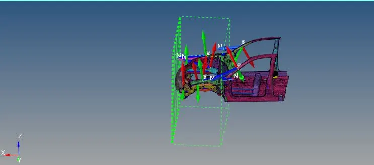
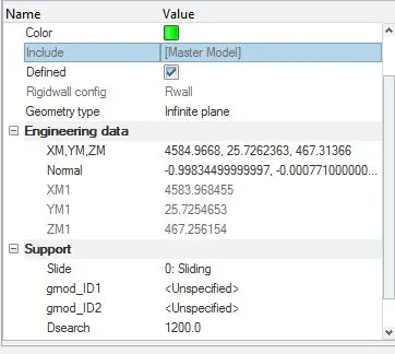
Fig 16 : Rigid wall definition Fig 17 : Prop card for the Rwall

1.6 Boundary conditions :

The boundary conditions for the problem is our automobile is moving at a velocity of 35mph. Converting it into the present unit system it is 15.65 mm/ms. The velocity is given to the total group of nodes as they will be moving at a velocity of towards the wall. The intial velocity condition is shown in the picture below.

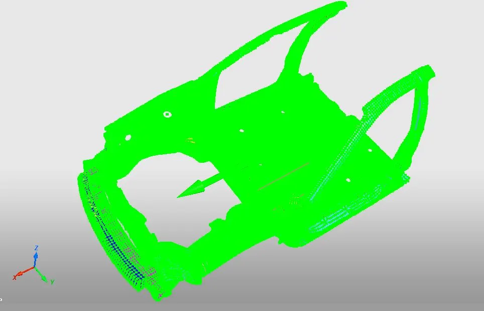
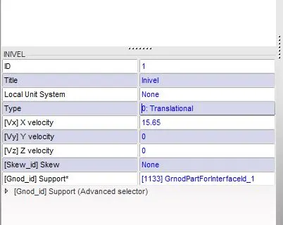
Fig 18 : Initial velocity Fig 19 : Intial velocity def

1.7 Section creation :

As said in the introduction there are few vital parts in the assembly of the BIW which take most of the impact loads. They include the shotgun(fender), rail, headlight bracket connected to the bumper, A pillar. The force generated at the contact of the wall and the bumper it transferred through the bumper and the headlight bracket then rail and fender and then finally to the A Pillar. The A pillar should ideally receive minimum amount of force. The rail should take most of the load. The pictures of those components and their connections are shown in the pictures below.

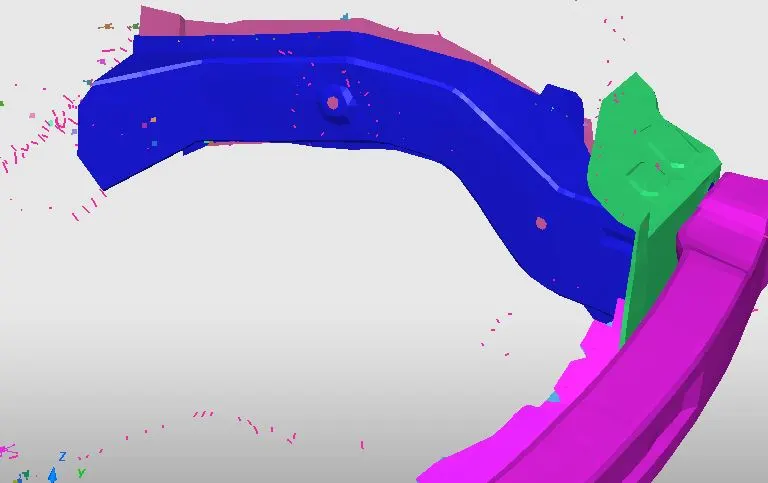
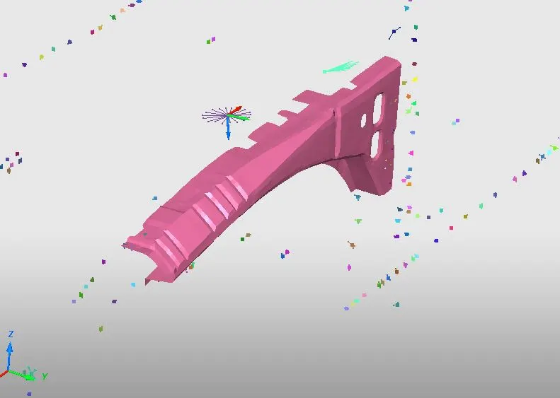
Fig 20: Left Rail Fig 21 : Shot gun

In order to study the sectional forces in the above mentioned parts sections need to be created. To create the section a moving frame is created initially and then the sections is created at the respective parts. The picture shows the frames created and then the sections. Care is taken that section is on xy plane. So individual sections are created at diff parts and the output requests for the resultant normal and the tangential forces are generated. The sections and their properties are shown in the picture below.

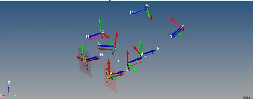
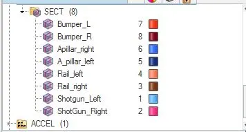
Fig 22 : Sections and moving frames Fig 23: Sections list

1.8 Accelerometer:

An accelerometer is created and is placed at the bottom of the B pillar to know the variation of acceleration with respect to time.

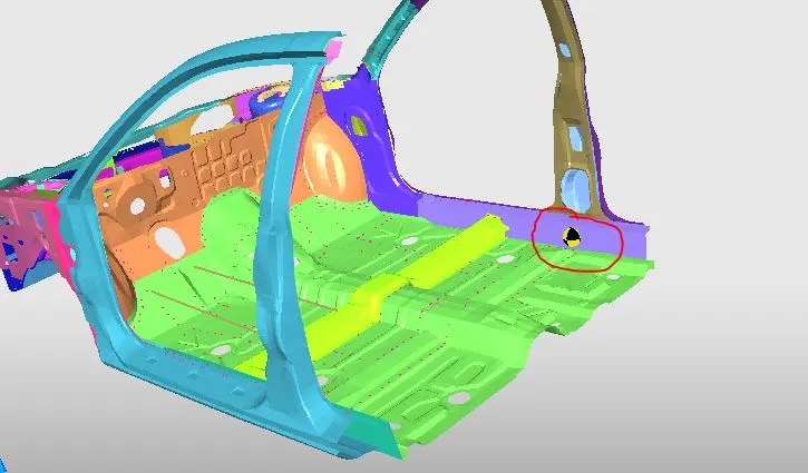
Fig 24 : Accelerometer

1.9 Nodal time step:

The time step need to be changed as per the required value. The change in the time step can be done using the DT/NODA card. The time step of 50micro sec is adjusted in the panel and it is converted to the required units ms,

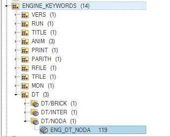
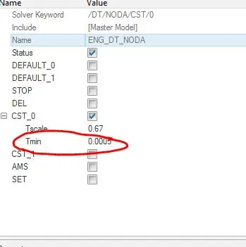
Fig 25 : Nodal timestep Fig 26 : Defining timestep

1.10 Intrusions :

The intrusion into the passenger cabin is very important parameter in the crash worthiness. The amount of the intrusion is measured with the help of two springs with minimum stiffness.

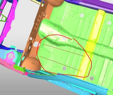
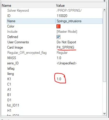
Fig 27 : Intrusion springs Fig 28 : Property intrusions

1.11 Output requests :

A total of 11 output requests are created to check the results. The output requests created will generate the data which is helpful later in plotting and understanding the physics. The output requests include acceleration, Normal and tangential forces at all the sections and at the rigid wall and the elongations of the intrusions were created.

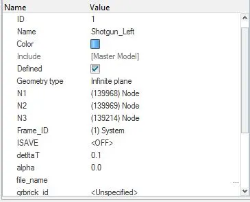
The picture below shows the position of the output requests in the tree and a sample request.

2. Model checking and debugging:

• To ensure that there are no errors we use model checker in the in hyper crash.
• We need to make certain that there are no penetrations and intersections in the contact interfacing and the components. This is done using penetration check in the tools option in Hypermesh.
• Two penetrations were found at the shock absorber housing and they were moved using the translate option in the tools,
• Most penetrations can be fixed automatically using auto fix option but the two penetrations here can only be set manually.
• Once the penetrations are fixed we can run the model checker and in the model checker the springs of the rigids near the shock absorber housing are shown as free.
• Those springs can be deleted and the now we have few warnings and no errors as long as we have no errors are ready to go.
• The pictures show the penetrations and the model checker and the manually removed error at the shock absorber housing.

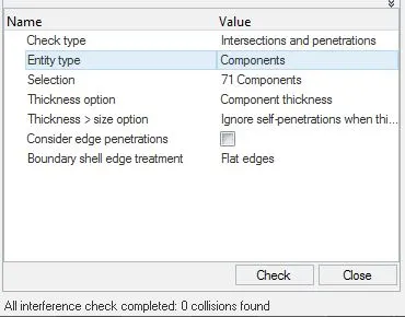
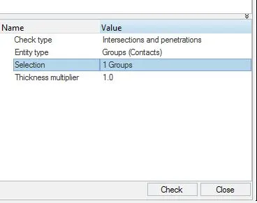
Fig 30: Component penetration check Fig 31 :Interface penetration check

Once the model is checked and ready to go we can start the radioss solver for the analysis.

3. Results and discussion:

3.1 Simulation:

The simulation shows the front crash of the neon model. The frontal crash on a barrier shows that the structural integrity of the neon model is good enough to take the crash. We did a crash analysis at 35mph and there is significant change in mechanics form left to the right.

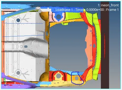
Fig 32 : Extra Hole

From the picture we can see that there is an extra hole present on the right side of the vehicle. The presence of the hole makes the right side of the crumple zone and that is the reason it crushes easily on the right side, whereas the left side remains slightly rigid. This can be clearly visualized form the pictures of the animation file below.

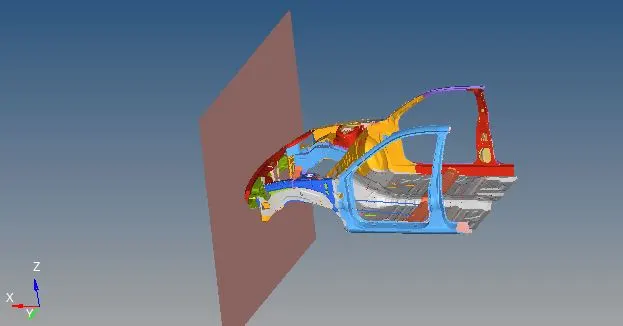
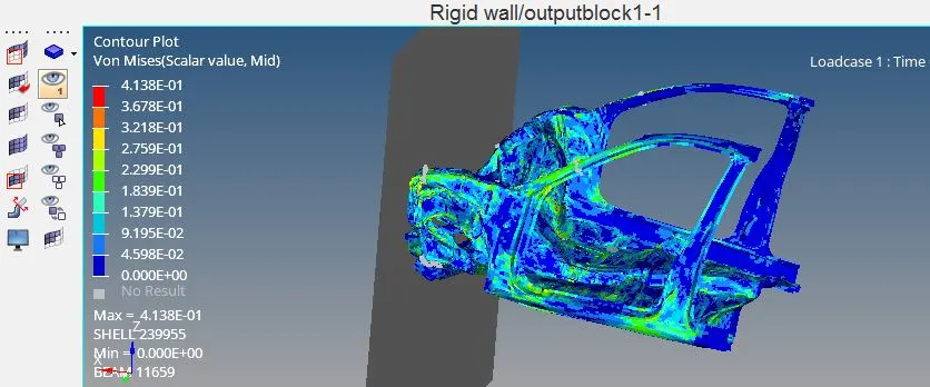
Fig 33 : Frontal crash Fig 34 : Vonmises stress distrubution

3.2 Shot Gun Forces:

3.2.1 Shotgun/Left

• The plot shows the force in KN on Y axis and the time in ms on Xaxis.
• As it is evident from the plot the forces peak at certain time, the reason is explained below.
• The value of force jumps up at certain locations near 30micro seconds and the 45microseconds.

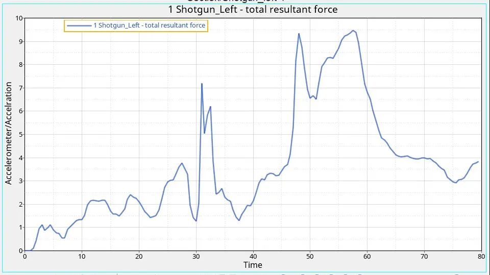
Fig 35 : Shotgun Left with respect to time

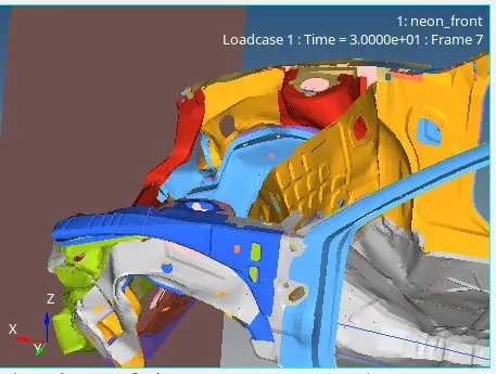
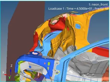
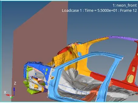
Fig 36 : Shot gun simulation at 30ms Fig 37: Shot gun left at 45 ms Fig 38 : Shotgun left at 55ms

• At 30 the shotgun just starts to collide with the rigid wall, due to this there is jump in the force
• Just before 40 ms the fender starts bending and it starts crushing this is where the force starts peaking and peaks to a value of 9.5 KN.
• And right after the 50ms the forces start to drop as the fender is comp0letly crushed the force drops.
• These statements were supported by the pictures at different times in the pictures below.

3.2.2 Shotgun/Right:

• The shotgun on the right side of the vehicle shows a significant variation in the forces and the crash behavior.
• This is due to the fact that the presence of the hole on the right side weakens the stiffness of the component.
• This generates a trend that is completely different to the left shotgun force trend.
• As we observe closely into the simulation and the plot we find certain things at 20ms the fender just starts colliding into the rigid wall.
• The force value peaks at this instant. Unlike the left shotgun the fender just starts crushing from this instant so there is no second peak after this point.
• The included screenshots of the simulation at different times reinforces the above explanation.
• Due to the hole the crush starts earlier in this case the hole plays a vital role in the trend of the shotgun forces.
• Maximum force of 7.3KN at 18ms.

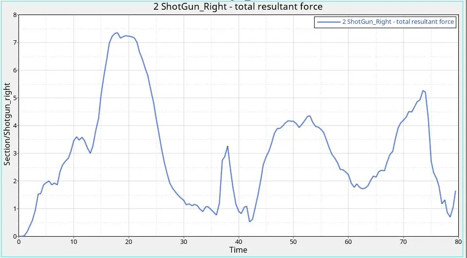
Fig 39 : Shotgun Right Plot wrto timestep

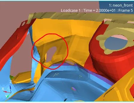
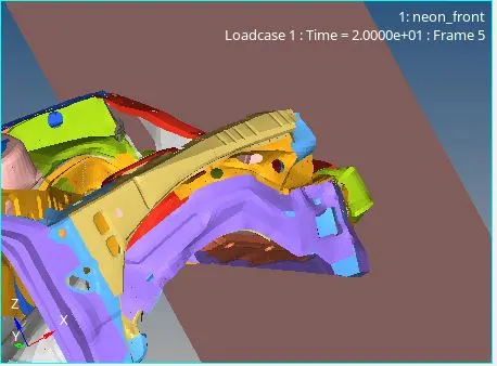
Fig 40: Impact of hole right shot gun 20 ms

3.3 Rail forces.

The rail is the sturdy component and it is designed to take up a major portion of the impact load. A detailed observation of the simulation and the plot gives important inferences.

3.3.1 Rail/Left:

• From the graph it is evident that the maximum force value occurs at 47ms and 13ms too.
• From the simulation we can see that the Rail starts colliding into the wall somewhere after 10ms and before 15ms that explains the peak in the forces
• After the initial impact the Rail starts buckling that is the reason why the force drops, and the buckled rail again collides with the wall which again increases the force at 45ms.
• So at 45ms the force again peaks up to 22.5KN.

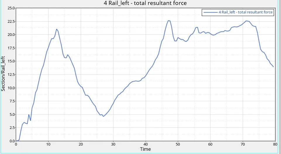
Fig 41 : Left Rail Force variation

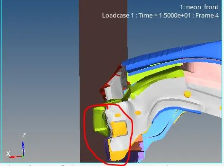
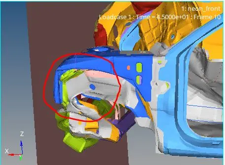
FIg 42 : left rail 15ms Fig 43 : Left rail 45ms

3.3.2 Rail/Right:

• From the simulation it is evident that the rail starts colliding with the wall near 9ms, so there is a peaking in the force until 5KN.
• As the collision progresses the force keeps on climbing up until the rail buckles i.e until 18ms. The force reaches upto
• The buckling of the rail; results in the reduction of the force, as the rail completely buckles and collision reaches the to 70ms where the bukled rail will collide again into the wall causing the maximum force in the rail i.e upto 26KN.
  

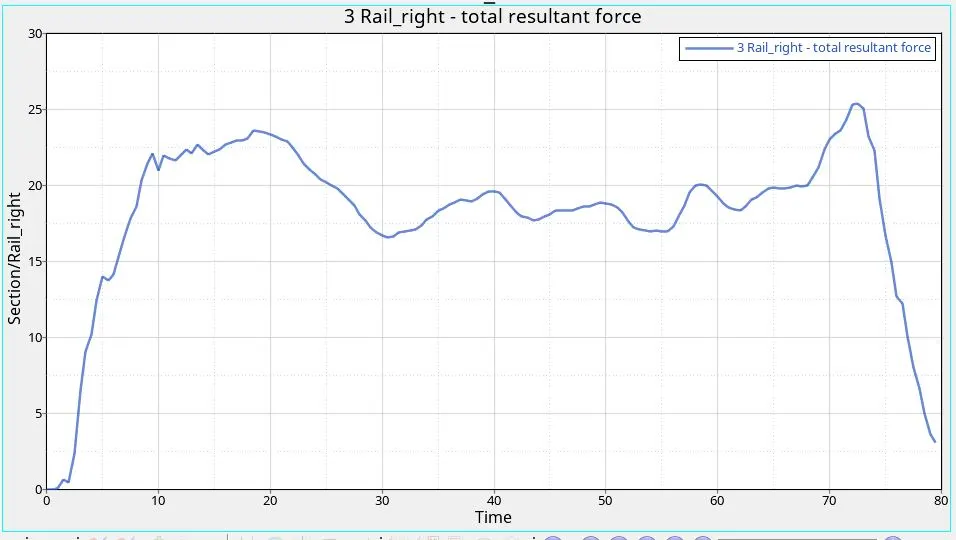
Fig 44 : Rail Right plot wrto time

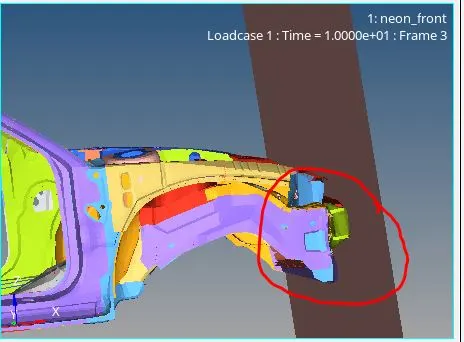
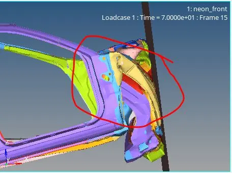
Fig 45 : Right rail 10ms Fig 46: Right rail 70ms

3.4 APillar forces:

The Apillar is a component which is the start of the cabin. Ideally Apillar should receive minimum amount of force as the passenger cabin starts form here. Due to presence of hole at the right side of the BIW there is significant variation in the crash behavior of the A Pillar on the left and the right.

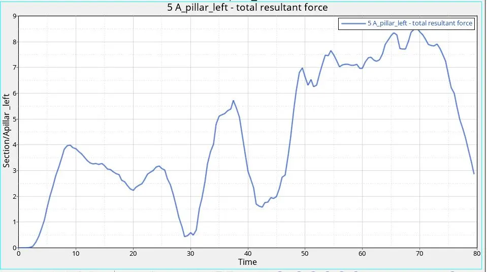
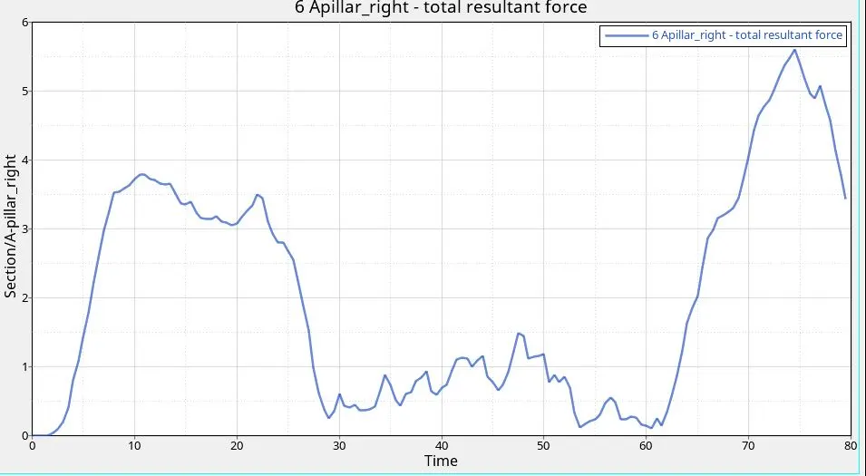
Fig 47 : A Pillar Left plot Fig 48 : A Pillar Right plot

3.4.1 A Pillar/Left:

• A Pillar left peaks at the end of the simulation near 70ms and the value of maximum force is 8.5KN.
• The A Pillar force plot and the simulation pictures are attached below.

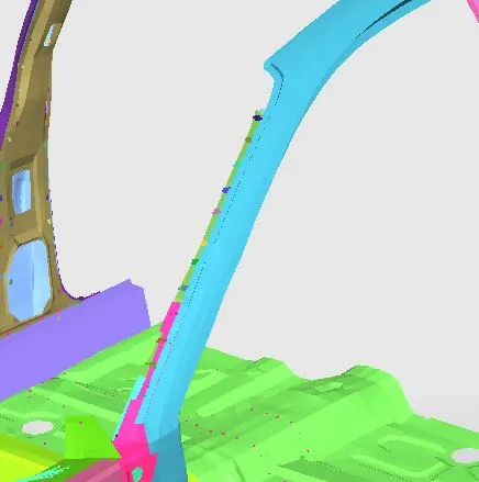
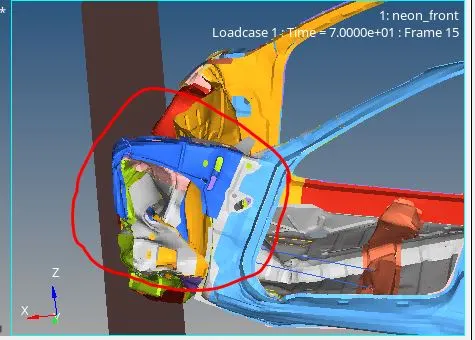
Fig 48 : A pillar Fig 49 : Simulation at 70ms

3.4.2 APillar/Right:

• A Pillar right has a maximum force of 5.5 KN at 75ms.

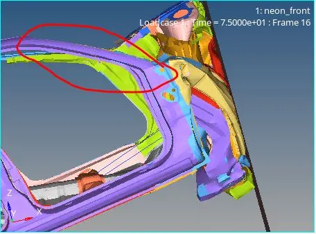
Fig 50: A Pillar Right 75 ms

3.5 Bumper forces.

The left and the right bumper forces are measured at the Head light brackets on either side. The maximum forces on the either side of the bracket are shown in the plots below.

Left: 12.3 KN at 10ms

Right : 10.5KN at 10ms

From the above observations we can infer that the maximum value of the force occurs in the rail.

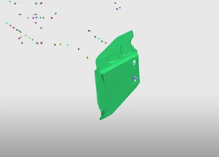
Fig : Bumper/ Headlight bracket

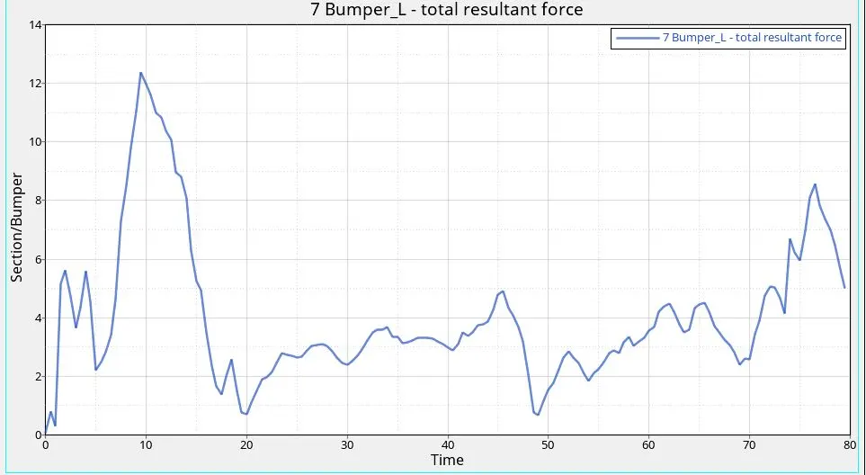
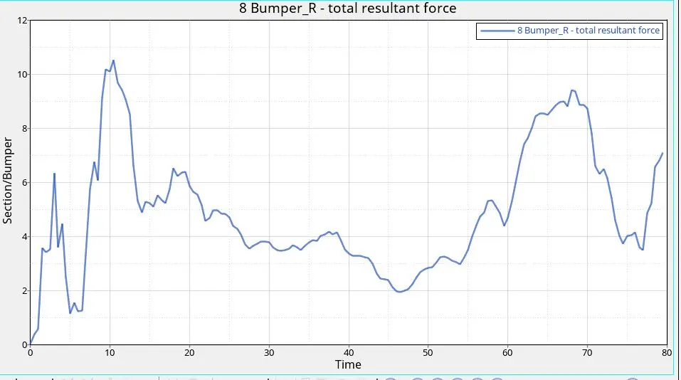
Fig 51 : Bumper Left plot Fig 52 : Bumper Right Plot

All the respective forces along with the wall normal forces are plotted on the same graph to understand the crash scenario holistically. The rigid wall forces peak up in the beginning as the crumble zone plays its part the rigid wall normal forces significantly drop. The crumble zone takes up lot of impact and the crushes there by reducing he impact. As the crash progresses the rigid wall forces lower down and the forces in the components increases and at the end the rigid wall forces again peak up to as the BIW completely crushes.

Crash worthiness depends on the amount of energy absorbed by the crumble zone and the transfer of the energy to the cabin area. The BIW shows decent crash worthiness as the Crumble zone absorbs most of the energy. The comparison of the R wall forces with the other forces on the left and right side of the vehicle is shown here below.

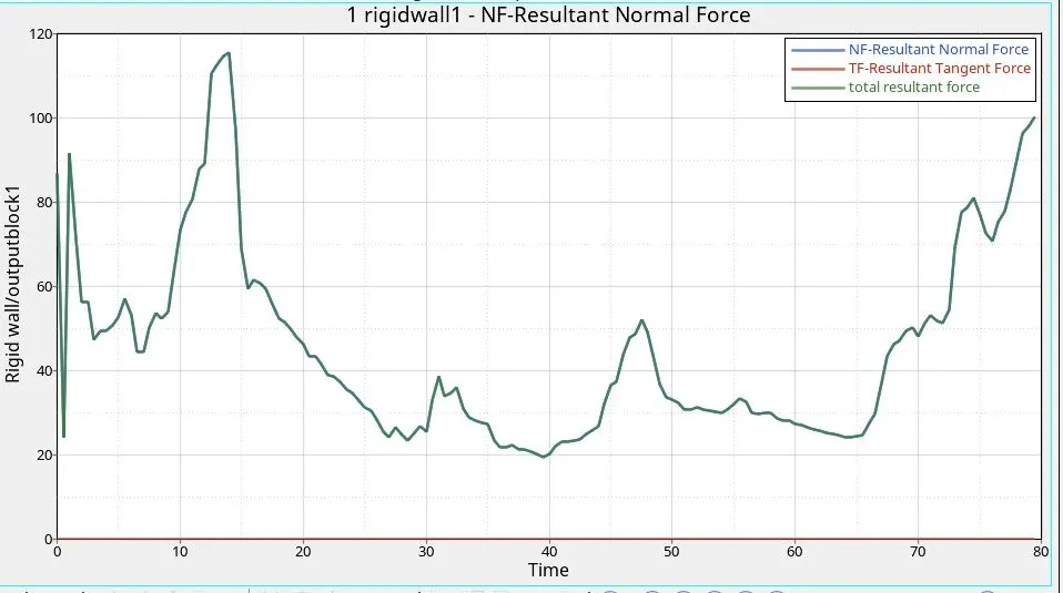
Fig 53 : R Wall resultant Normal Forces

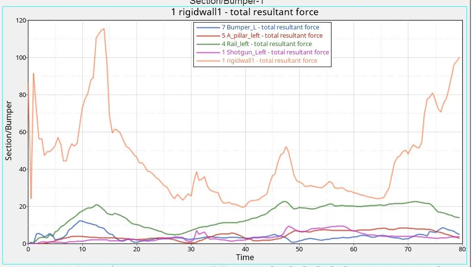
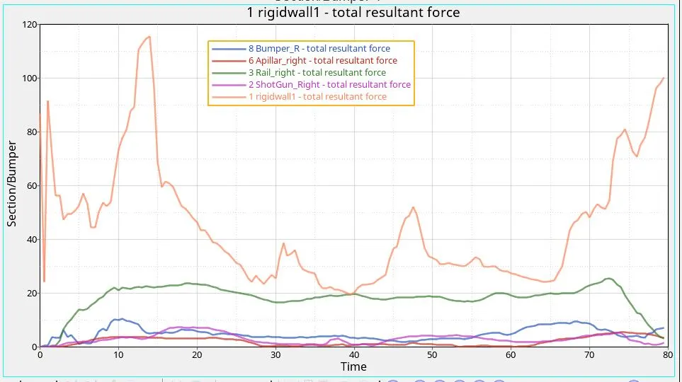
Fig 54 : Rwall Normal and all the left components Normal forces Fig 55: Rwall and all the right compnent normal forces

3.6 Accelerometer:

An accelerometer is arranged at the base of the B Pillar to measure the acceleration during the crash. The peak value of acceleration occurs at the 68ms and the value of maximum acceleration is 1.83mm/ms2.

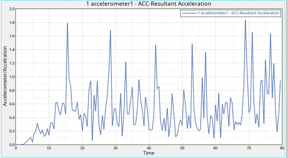
Fig 56: Accelerometer acceleration curve

3.7 Intrusions:

The Intrusion is a key parameter in the crash analysis. The amount of intrusion shows how much passenger cabin is affected by the impact. The intrusions are measured using two springs with negligible stiffness of 1KN/mm. They were installed at the respective nodes as asked. The variation of the elongation is measured and were plotted with respect to time.

A negative elongation in the x direction is shown wrto time as the spring is compressing. A total of 5mm is observed along the for the intrusions. The variation in the elongation for both the springs and their plots are given below.

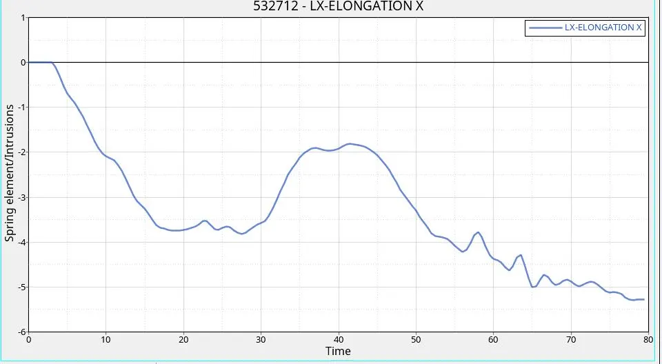
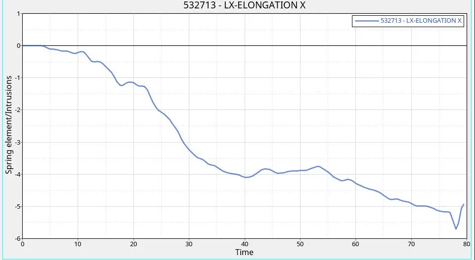
Fig 57 : Displacement of the farleft spring Fig 58 : Displacement of the spring towards the dasboard

3.8 Out file:

The output file shows the time step which is 0.5 micro seconds, the energy error is under check and does not exceed 3percent which is good indication that not much of hourglass energy is created. The mass error is also under control and not mass addition algorithm needed. The picture shows the outfile which showcases the time step value and the energy, mass errors.

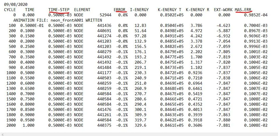
Fig 59: Output file

The front crash analysis is performed on a neon dodge BIW. The crash behavior and the impact analysis on different components is done. The load distribution at different sections of the BIW is inferred using different output requests. The physics of the crash of an automobile is understood with the help of simulation and the graphs. Contact modeling and setting up a frontal crash from defining boundary conditions to extracting outputs is thoroughly understood as part of the project 1.

Please find the attached files in the zip file challenge.zip