Assignment 5-RADIOSS Interfaces & Study of Effect of Notches Challenge

Assignment 5-RADIOSS Interfaces & Study of Effect of Notches Challenge

1. Meshing of Bumper Assembly

A CAD model of the bumber was provided and it was asked to mesh it with a 6mm mesh size. The geometry is shown in the attached figure. It was clear that this is only half a portion of the bumper model and we need to use reflect tool to obtain the other half of the model.

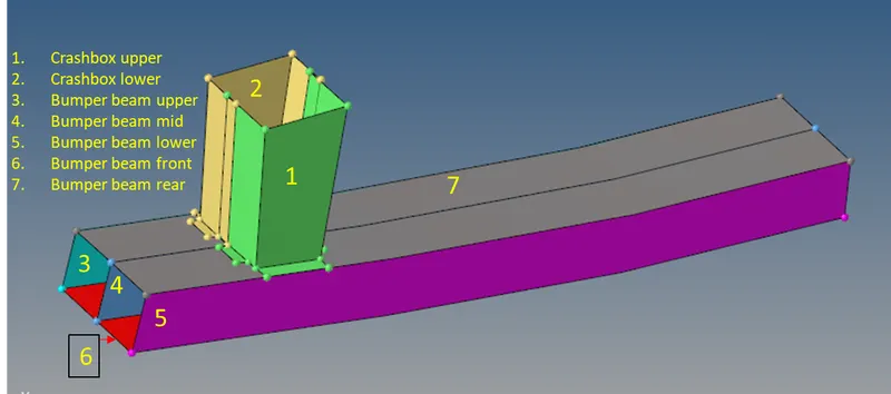
Fig 1.1: The bumper model

The first step was to perform the geometry cleanup of the model. All the surfaces were joined properly using the surface edit tools and quick edit commands like replacing points. After that quality criteria was selected as shown in the attached figure.

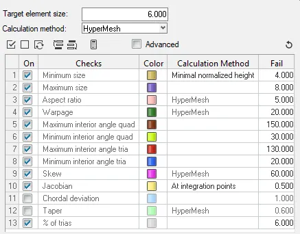
Fig 1.2 The quality criteria followed for the mesh

After that mesh was generated on the surface using a mixed type of elements. Tria elements were removed using the cleanup tools available in the quality index menu.

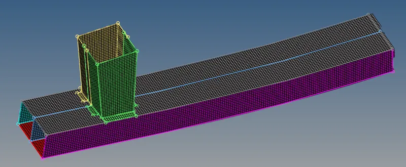
Fig 1.3: The meshed half portion of the bumper assembly

After that spot weld was used to join the crash box components with the beam components. ACM (shell gap contact+coating) was used as the type of element. It uses a hex element per connection and links it to the shell elements.

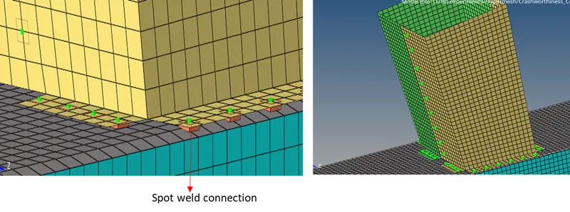
Fig 1.4: the spot weld connection used for the model

Then the elements were reflected as shown in the below-attached figure. The connectors were reflected separately and realized again.

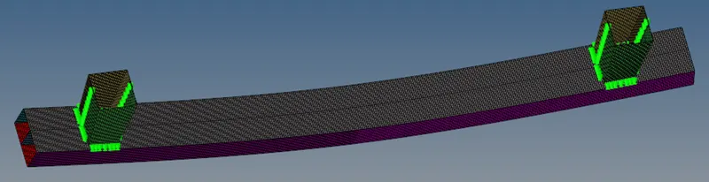
Fig 1.5: The completely meshed model

2. Study of interface modelling in Radioss

Interfaces or contacts are defined to model how the parts have when they come into contact with each other. They affect the timestep and also introduce non-linearity into the system. The study of an interface or contact mainly involves understanding three things:

• Method- The penalty method is the most commonly used one
• Stiffness Formulation- The Penalty method treats the behaviour between slave nodes and the master segment as a spring element that generates resistive forces as a function of penetration. The nature of stiffness can be linear or non-linear depending upon the type of contact used.
• Type of Interaction- Any contact works by defining master and slave entities. Based upon the entity selected for master and slave a contact can be: (a) Node to Surface (b) Edge to Edge (c) Surface to surface.

The penalty method creates a spring element between the slave node and its projection. The spring stiffness is automatically computed according to the material and properties of master and slave nodes. The resistive force generated by the imaginary spring is called an interface force. As soon as the slave node gets inside the gap (defined volume), it begins to experience spring force of contact.

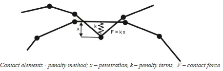
Fig 2.1: Representation of the penalty method

The stiffness of the spring depends on material bulk modulus K, face area A, volume V or shell diagonal and a numerically selected scale factor f ; `k= f* (KA^2)/V`

Further, the modeller needs to take care of initial penetration while doing the meshing. Certain algorithms are there which can deal with it but in the cases, it is too much and can be called an intersection, it leads to failure of the solution.

Some of the contact methods available in the Radioss are shown in the below table:

Type 2	Tied node to surface
Type 3	Surface to Surface
Type 5	Node to surface
Type 6	Special rigid body to rigid body
Type 7	General node to surface
Type 10	Tied node to surface after impact
Type 11	Edge to edge
Type 14	Madymo ellipsoidal to node
Type 15	Madymo ellipsoidal to node
Type 19	Type 7+ Type 11
Type 20	General Contact
Type 23	Special self-impact contact for airbag
Type 24	General node and surface to surface

Table 2.1: Available contact types in Radioss.

There are some recommended settings for most of the contacts used in the Radioss. They can be used to model an accurate contact for crash applications.

Parameter	Comment
------	Remove all the intersections or initial penetrations that are due to inaccurate meshing in a pre-processor
Igap =2	Set Variable gap to take into account all the true distance between parts
Gap (min)>=0.5	Specify the minimum thickness of the model to avoid the numerical issue. Typically half of the thinnest part in the contact
Inacti=6	Remove initial penetration wherever possible, elsewhere reduce to less than 30% of the defined gap value and adjust the gap with Inacti
Istf= 4	Set stiffness of the interface base on the softer of the master and slave
Stmin=1000N/mm (say)	Specify a minimum stiffness in the contact to avoid too soft contact
Idel=2	Remove slave nodes from contact because of contact element deletion
Iform=2	Sliding forces are computed using stiffness parameters of the contact
------	Define physical values for the material constants and part thickness, even if the component is a rigid body. They are used for calculating gap stiffness and gap definition

In this assignment, a crush tube model was tested with different types of contact algorithms and a notches model. The detailed statement is presented below:

1. Run the crash tube model as it is.
2. Change the Inacti=6 and run.
3. Create the type 11 contact and run.
4. Remove both notches and remove boundary condition on rigid body node then run.
5. Create a new notch in the middle, select the whole section and run.
6. Create a new notch with nodes only from opposing 2 faces and run.

Note:

• Plot RWALL forces, contact forces, internal energy and Create TH/PART for all parts and compare results for all cases.
• Comment your thought on why there is a change in the internal energies.
• How does the notch affect the results?
• Plot energies and note any difference.

3. The provided model Crush Tube model

A Radioss solver deck file was provided as part of this assignment. The file contains meshed model along with all the necessary cards for a simulation. They are discussed one by one in the following sections:

3.1 The Model:

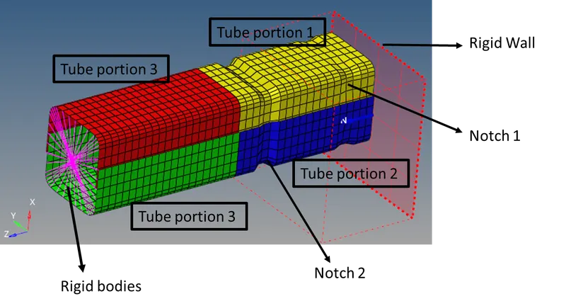
Fig 3.1.1: The geometry of the model

Four C shaped portions are meshed with shell elements and are connected together with Type 2 contact and a spider of rigid elements at the rear end as shown in the attached figure above. A rigidwall is modelled in the front to which the crush tube is going to crash. For the boundary condition, a velocity of 13.3 [mm/ms] was provided to all nodes of the model. This was imparted using the INIVEL card as shown in the below-attached figure.

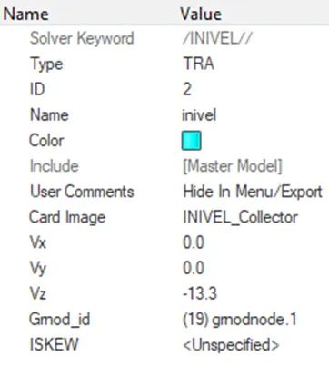
Fig 3.1.2: The INVEL card used to assign velocity to the nodes

3.2 Material and Section Properties

Shell section properties were assigned with thickness values as shown in the attached figure. Ishell =24 was used to enable QEPH shell formulation. N=5 was used to get 5 integration points through-thickness.

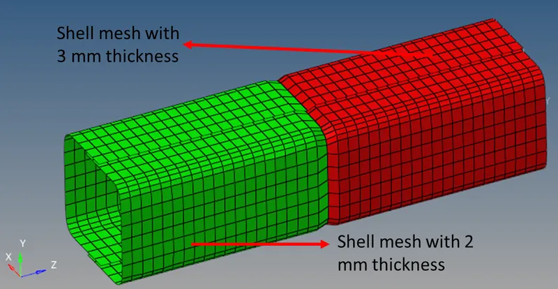
Fig 3.2.1: Shell properties assigned to different components

Steel was used as a material for the components. The law 2 card was used, this law represents an isotropic elastoplastic material using the Johnson-Cook material model. This model expresses material stress as a function of strain, strain rate and temperature. A built-in failure criterion based on the maximum plastic strain is available. The material card is shown in the below-attached figure.

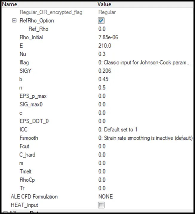
Fig 3.2.2: The material model used

3.3 Contacts used in the model

Initially, the model contains two contacts for different components of the model. They are type 2 and type 7 contacts. The type 2 contact is used to model spot weld for the components and type 7 is used to define a self contact between the components so that they do not penetrate each other during buckling.

Type 2 contact/ Interface

It defines a TYPE2 tied interface that connects a set of slave nodes to a master surface. It can be used to connect coarse and fine meshes, model spot welds, rivets, and so on. A group of nodes from the outer surface at joints was used as slave and elements from the underlying mesh was used as surface (made into a set using the Surface segment keyword).

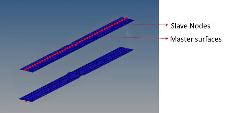
Fig 3.3.1: The type 2 contact used to model spot weld connection

The dsearch value was kept at 5 mm which tells the solver to look for the closest master segment. Other than that, all the parameters were kept default.

Type 7 Contact

Interface TYPE7 is a multi-usage impact interface, modelling contact between a master surface and a group of slave nodes. It is also possible to consider heat transfer and heat friction. Its best use case is for defining self contact for components of a model. There are some disadvantages of type 7 contact. It does not tolerate intersections (slave node penetrating into the master segment). Also, timestep may reduce due to increasing interface stiffness.

Sometimes the node to surface scheme fails to detect a contact even if the edges of the master and slave elements have intersected each other due to edges crossing each other at angles. This can be avoided by adding an additional Type 11 which is an edge to edge type of contact.

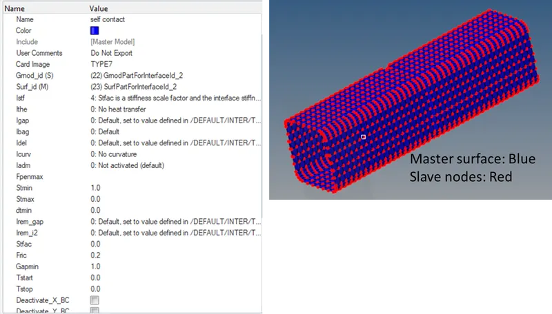
Fig 3.3.2: The type 7 Contact used in the model

3.4 Engine cards and output requests

Termination time of 30 ms was defined using the /RUN card and /ANIM/DT card was used to request animation files at a frequency of 1ms. Apart from this, /ANIM/VECT card was used. It generates animation files containing vectorial data for the specified variable. In this case, velocity, contact forces, forces and moments for rigid bodies, rigid walls and sections and displacement data were requested. Similarly, ANIM/NODA card was used to write animation files containing nodal scalar data.

We need to add the time history keyword /TH or /Tfile to be able to get the T01 file written by the solver. This file is input to the Hypergraph where all the plots can be generated. In this model following /TH keywords were used:

• /TH/NODE: to record the time history of the independent node of the rigid spider at the rear end.
• /TH/INTER: This card was used to required to enable the recording of time-history data for all the interfaces/ contacts in the model.

As discussed in section 2, a total of 6 cases were simulated for this exercise. They are discussed one by one in the following sections:

4. Results and Discussion

4.1 Run the crash tube model as it is.

The solver deck file was imported and was run using the Radioss solver.

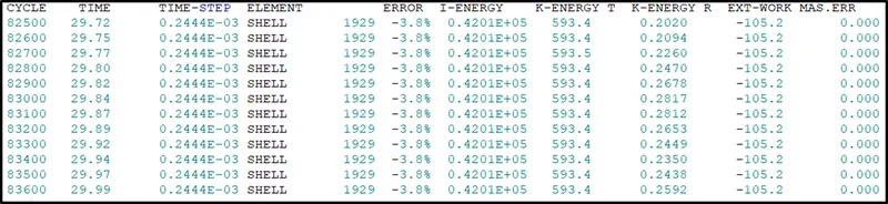
Fig 4.1.1: The snapshot from .out file showing energy and mass errors.

The induced energy was 3.8% and there was no mass error in calculations. The total time taken to run the simulation was 232.89 s.

Animation 4.1.1: The crush tube simulation

As clear from the animation the notch acts as a point of buckling initiation. This happens due to stress concentration in the notch regions. Also, the contacts are working fine as we don't observe any separation of edges joined with type 2 contact and there was no apparent self penetration by elements from the same component.

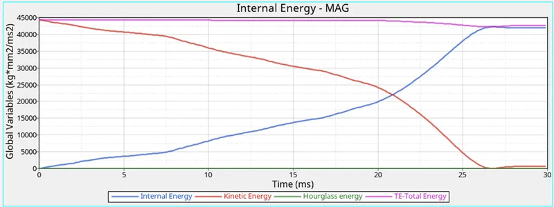
Fig 4.1.2: The energy plots for the case

The energy plots resemble that of a typical crash test and hourglass energy is negligible as seen in the plot. After the contact between the tube and the rigid wall, the Kinetic energy begins to fall with a rise in Internal energy. The total energy remains almost constant with little fluctuation. After 21 ms the IE and KE plots cross each other and finally, KE becomes zero and IE becomes equal to Total energy.

After energy plots, we need to examine the Rigidwall forces. The plots for the rigid wall forces are shown in the below-attached figure.

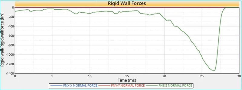
Fig 4.1.3: The plot for normal forces on rigidwall

The normal force in the Z direction is the only significant one and after peaking at almost 27 ms it goes back to zero signifying complete deformation.

Next, we need to check the forces on interfaces one by one. This data was requested using the /TH/INTER card as discussed in section 3.4.

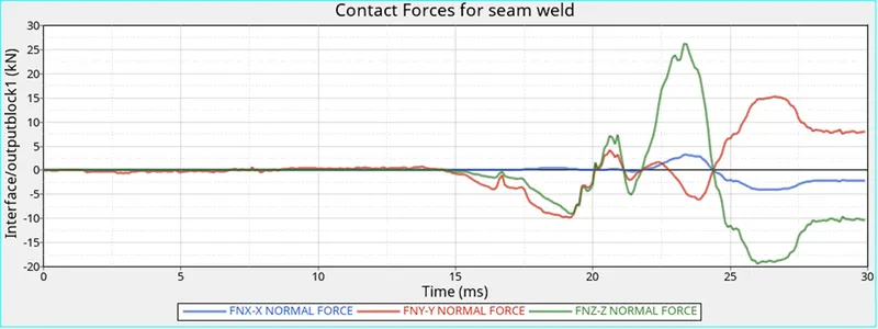
Fig 4.1.4: The Normal contact forces at the seam weld or type 2 contact

The plot becomes suddenly noisy after 15 ms, this is due to the rapid buckling of the rear portion after the two components at the front have buckled completely.

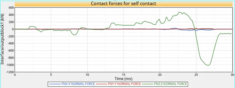
Fig 4.1.5: The contact forces for the self contact or type 7 contact

The nature of Z force variation matches that of the Z normal force in the plot for type 2 contact. A similar argument can be made about the variation of the forces.

4.2 Change the Inacti=6 and run.

The value of Inacti in a contact card dictates how to deal with the initial penetration in the model. The initial penetration may be the result of improper meshing and it is recommended to avoid it from the meshing stage itself. Basically, initial penetration results when slave nodes go past the master segment. This can lead to locking and lead to failure of computation.

Inacti	Action	Remark
0	No action	Best option (if possible)
1	De-activation of the node stiffness	Low accuracy (Creates holes in the contact)
2	De-activation of the master stiffness	Low accuracy (Creates holes in the contact)
3	Automatic removal of the initial penetration	Dangerous - may alter the model
5	The gap is reduced	Good accuracy
6	The gap is reduced and scaled	Good accuracy

Option 6 is the best choice as it offers a reliable solution at a lesser CPU use during simulation. So, the Interface card was modified as shown in the attached figure.

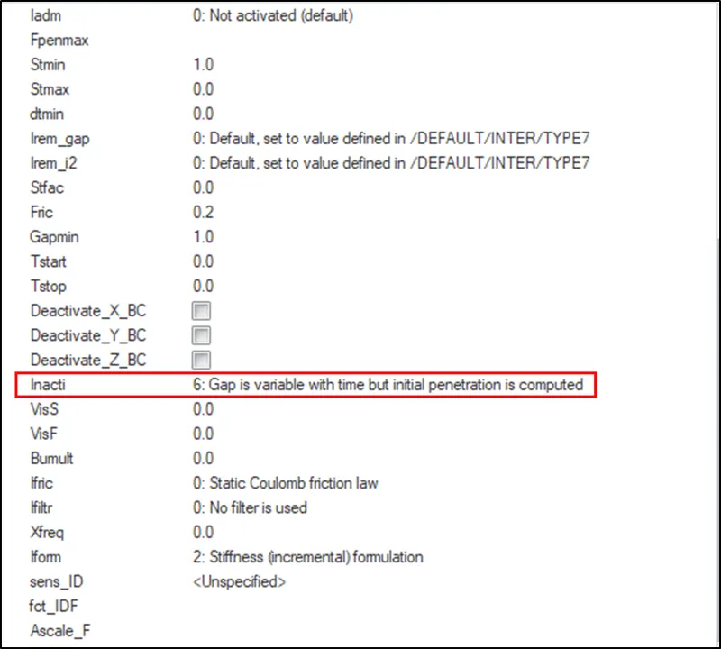
Fig 4.2.1: The snapshot from Type 7 interface card

Effects

The energy error induced in the model is still 3.8% as clear from the below-attached figure.

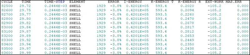
Fig 4.2.2: The snapshot from .out file showing computation data

The total time taken to complete the simulation was 233.42 s which is almost the same as the previous case. So far there is not much difference in solver time and errors. Next, we need to check different plots to be able to do a comparison.

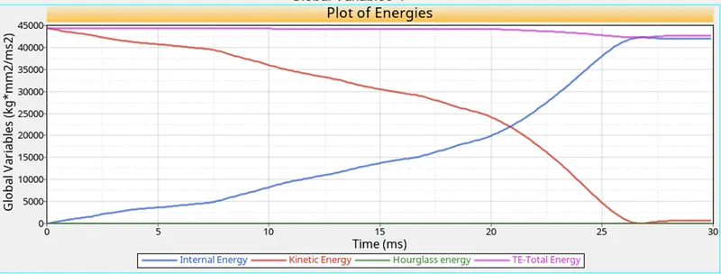
Fig 4.2.3: The plot of energies for the case with Inacti= 6 in the contact card

The energy plot is similar to the previous case without much change and a similar argument can be made for this case as well. There was no initial penetration in the model so we do not expect many changes in the results. It is a simple model but with complex assemblies containing multiple parts, the probability of initial penetration becomes high.

Fig 4.2.4: The plot of Rigid wall forces for the case with Inacti being set to 6

Similar to the earlier case, the Z normal force peaks after about 22 ms and retracts to zero value by 27.5 ms. This peak formation is due to the contact of the independent node of the rigid spider with buckled tube sections.

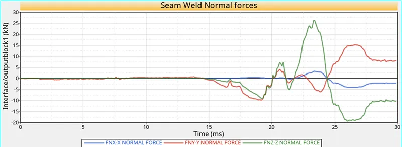
Fig 4.2.5: The plot of normal forces for type 2 (seam weld) contact

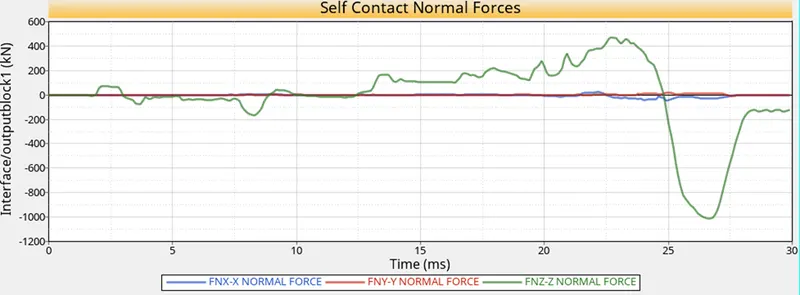
Fig 4.2.6: The normal forces for self contact used in the model

There is no apparent difference in the forces when compared to the results from the previous case. The explanation from the previous section holds good for this case as well.

4.3 Create a type 11 contact and run the model.

Type 11 contact is an edge to edge contact which simulates impact between edges to Edge or lines. A line can be a beam or truss element or a shell edge or spring element. Type 7 contact (node to surface) fails to detect contact in the events of edges crossing at an angle and bigger element sizes. This problem can be eliminated with the use of type 11 contact in addition to type 7 contact. Type 11 contact is defined by identifying master and slave lines (Edges). It works similar to type 7 in terms of penalty formulation, gap definition and search method.

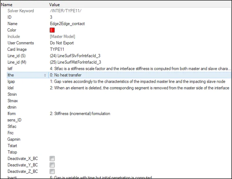
Fig 4.3.1: The type 11 contact details

It was defined by selecting the master and slave using components and all the components were selected for both. The results are discussed below:

Animation 4.3.1: the simulation of the crush tube with type 11 contact

The crushing of the tube looks similar in the animation and not much difference can be found.

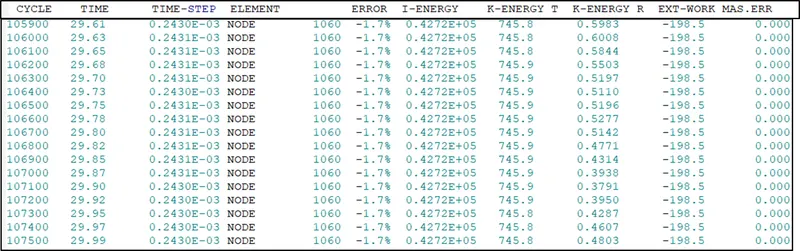
Fig 4.3.2: The output message file for the simulation

This time the energy error falls to 1.7% which is a significant drop and the accuracy of the simulation can be expected to be better this time.

The time taken to run the simulation this time is 586.74 which is an increase of 152 %. So adding this contact increases the computational resources significantly.

Next, we need to take a look at the plots for this model as done in the earlier cases.

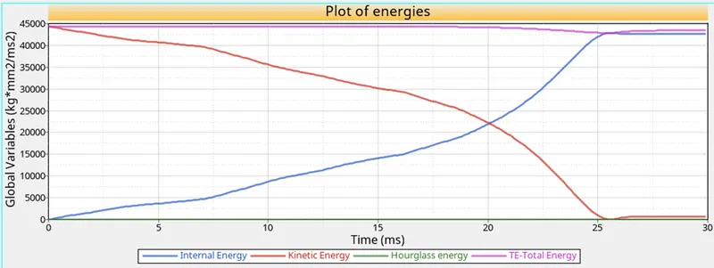
Fig 4.3.3: The energy plot for the case with type 11 contact

The notable difference is that the IE and KE lines are meeting earlier as compared to the previous cases. This can be due to the fact that after edge to edge contact the interference or disturbance to the buckling due to elements from the same component was reduced and the process was somewhat accelerated. Apart from this, the trends remain the same.

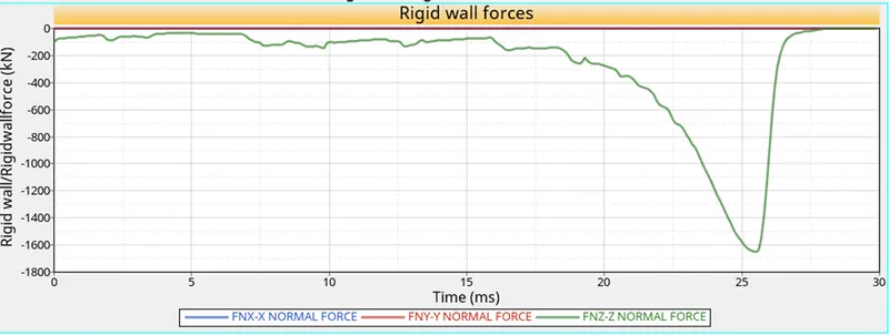
Fig 4.3.4: The plot of normal forces on the rigid wall for the case with type 11 contact in the moel

Again the trend remains the same and there is a little bit of shifting in the peak. The same argument applies to it, as disturbances due to self contact were reduced, and the buckling was accelerated.

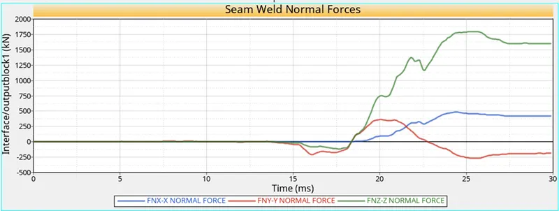
Fig 4.3.5: the normal forces developed in seam weld contact

This time the fluctuation has reduced and After changing the sign the Z normal force goes on increasing with little corrections in the way before coming to a constant value. This can be attributed to the fact that the seam weld joint or connection bears more force in comparison to earlier cases. Previously interferences or penetrations that go undetected by the type 7 contact were causing changes to the load born by seam weld in an unrealistic manner.

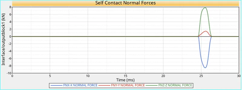
Fig 4.3.6: the normal forces generated due to self contact

The plot is petty simple and indicates self contact happened after a certain amount of buckling. This can be confirmed from the animation also, right after the collapse of notch, the elements begin to pile up and this led to the bubble-like shape at about 25 ms.

4.4 Remove both notches and remove the boundary condition on the rigid body then run the simulation

The notch was removed using the node align tool available in the geometry panel of Hypermesh. The process is shown in the below-attached figure.

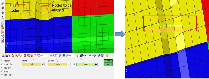
Fig 4.4.1: The process of notch removal

This step can be repeated to get all the nodes on the surface. It is a time-consuming process. A better way to get it done is by using the FE to surface tool from the surface menu and then repairing them to get a notch-free surface. Later on, the elements can be projected to the surface using the project tool available in the tool panel.

The constraint on the rigid body was removed by deleting the BC card used in the model.

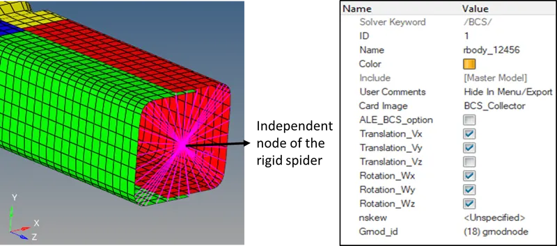
Fig 4.4.2: The boundary condition applied to the independent node of the rigid spider

As clear from the above figure, the independent node was restricted to only translate in the Z direction. All the remaining DOFs were arrested.

This card was deleted and the simulation was run. The results are discussed below:

The energy error this time was just 0.1 %. A reduction can be there due to the free movement of the crush tube upon impact as the restriction on the rigid body was removed.

Animation: The simulation without notch and constraints on the rigid body

The crush tube can be seen bouncing off at the end of buckling, this is the effect of constraint removal from the independent node of the rigid body. Next, we need to examine various plots obtained using the hypergraph.

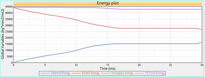
Fig 4.4.3: The energy plot for the case with the notch removed and no constraint on the rigid body

The energy plot is different this time. The plot can be divided into two portions, the first one is up to 16 ms and is similar to the earlier case. IE and KE are converging, but after that, the lines remain straight signifying the loss in contact or bouncing of the crush tube. Towards the end again the lines can be seen converging which implies re-contact of the crush tube with the rig wall.

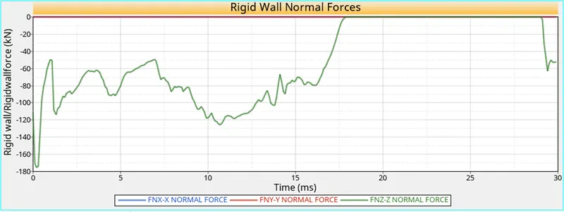
Fig 4.4.4: The plot for rigidwall normal forces

The bouncing off of the crush tube is reflected by Z normal force reducing to zero at about 17.5 ms. Apart from that, the data is noisy and there are corrections involved which may be due to the self contact and the edge to edge contacts present in the model.

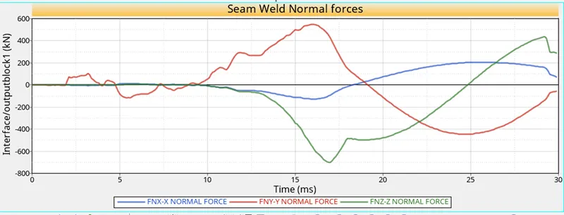
Fig 4.4.5: The normal forces on the seam weld connection

The Z normal force changes its sign at 25 ms and at this time the tube is not in contact with the rigid wall, so it can be due to a change in orientation of the tube as it bounces off.

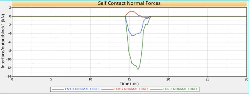
Fig 4.4.6: The self contact normal forces plot

Again the nature of the plots is the same as that of the earlier ones and a similar bubble-like shape can be observed at around 15 ms.

4.5 Create a new notch in the middle, select the whole section and run

The process of making a new notch involves translating two rows of nodes in the middle by 2.5 mm as shown in the attached figure.

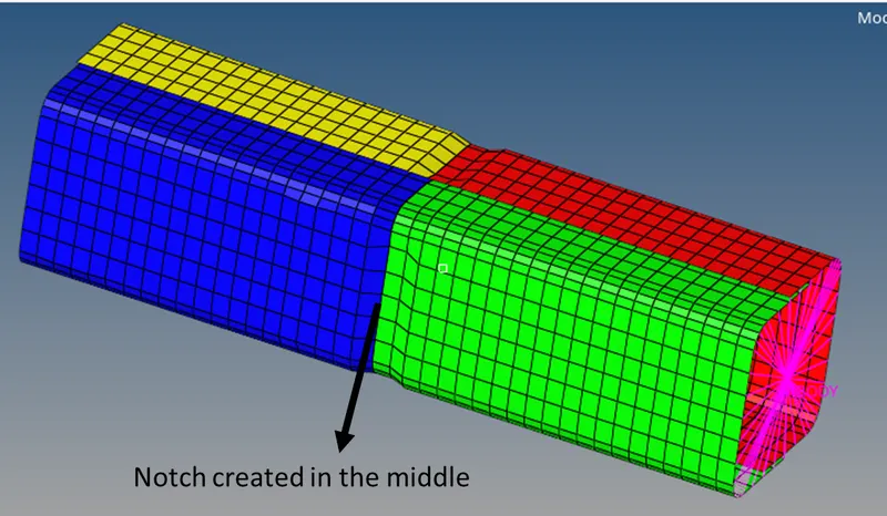
Fig 4.5.1: The notch created in the middle

After this, the simulation was run and the results are discussed below:

The energy error this time was -1.5% and the simulation time was 584.14 s. The energy error is more in comparison to the previous case, this signifies more simple the geometry, the lesser is the energy error. Features like notches have an adverse effect on the overall energy balance.

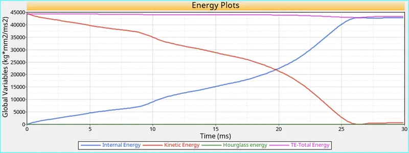
Fig 4.5.2: The energy plot for the case with a notch in the middle

This is the same as the cases with notches in the tube. So all the explanation holds good this time as well.

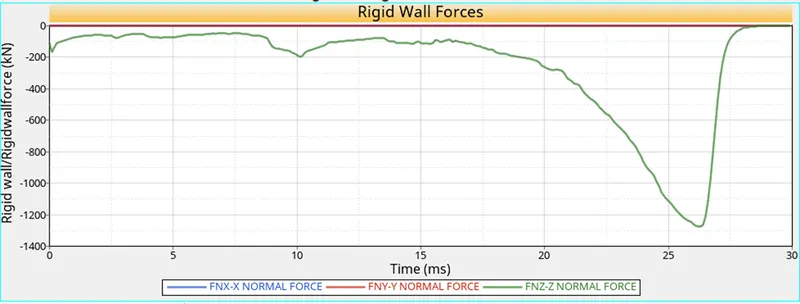
Fig 4.5.3: The normal rigid wall forces

Again the trend is the same and a similar explanation can be given for this as well.

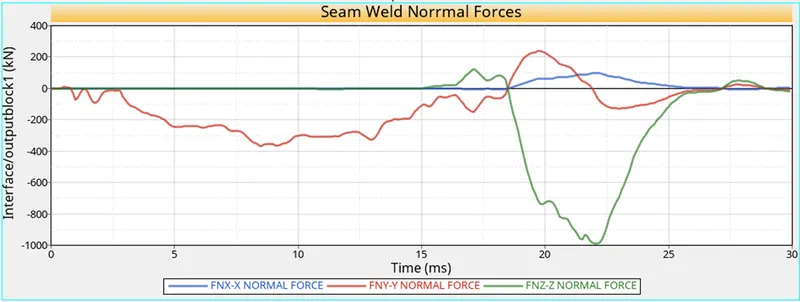
Fig 4.5.4: The normal forces on the seam weld connection

The plot this time looks more in this case, this can be explained by the fact that this time the notch is present at the location where different tubes are meeting which weakens it further. This leads to a greater force being experienced by the seam weld joint.

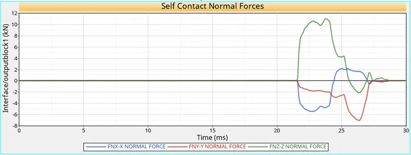
Fig 4.5.5: The self contact normal forces

The overall trend is similar for the normal forces, although the magnitude this time is higher.

4.6 Create a new notch in the middle with nodes from the opposing two faces only.

This case is much similar to the previous one. This time the notch created in the midllle was made of single row of nodes from the opposing faces as shown in the below-attached figure.

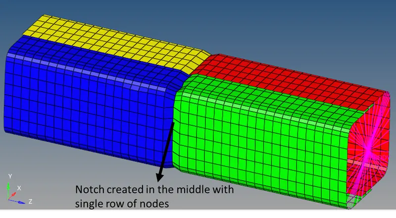
Fig 4.6.1: The notch created in the middle

All other keywords were kept the same and the simulation was run. The results are discussed below:

The energy error this time was -1.6%. Also the time taken to complete the simulation was 528 s. These two figures are in the sam ballpark, so all the previous explanations hold good.

Animation: The case with notch in the middle made from the nodes of opposite faces only

Stress concentration at the notch can be seen clearly and it acclerates the buckling process. Next, we need to take a look at the plots obtained from the hypergraph.

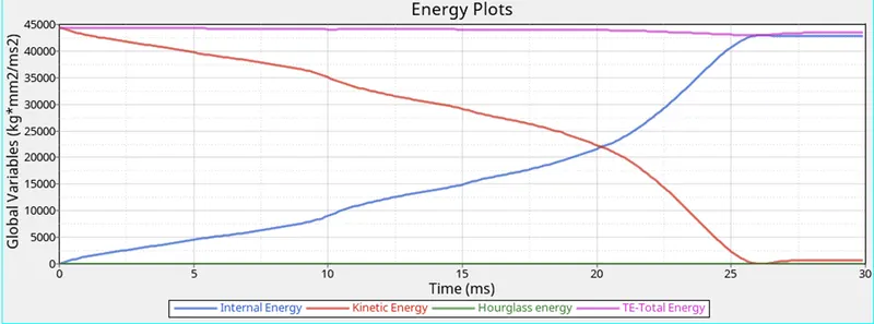
Fig 4.6.2: The energy plot for the case with notch made of nodes from the opposite faces only

There is no any remarkable difference in the energy plots, so all the explanations hold good for this one also.

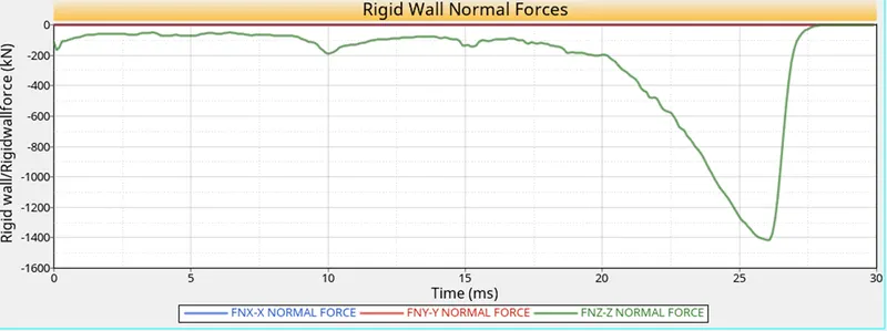
Fig 4.6.3: The rigid wall normal forces plot for the case with notch made of nodes from the opposite faces only

Again the plot is similar to the earlier cases and can be explained based on the previous statements.

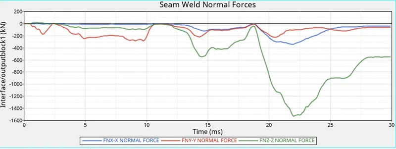
Fig 4.6.4: the normal forces on the seam weld

There is a greater magnitude present in this case, This may be due to the fact that a more sharp notch is present in the model leading to higher stress concentration. This weakens the structure further as compared to the previous case.

5. Conclusion

• A seam weld connection can be modelled efficiently in Radioss using a Type 2 contact.
• A type 7 contact (Self contact) can be aided by using an additional type 11 contact. This enables to capture the self intersections in a much efficient manner.
• Notches lead to stress concentration and represent the wekest portion.
• Use of Type 11 contact (edge to edge) increases the time taken to complete the simulation significantly.