Assignment 4-RADIOSS Material Laws Challenge

AIM : RADIOSS Material Laws Challenge.

OBJECTIVE : Run the model in RADIOSS as per the required parameters and compare them using the plots and animations

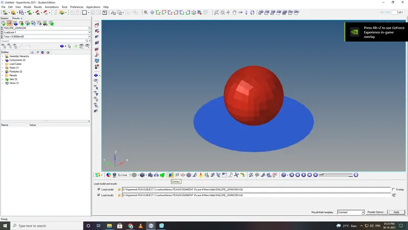
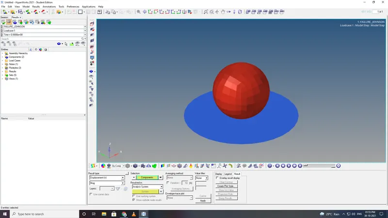
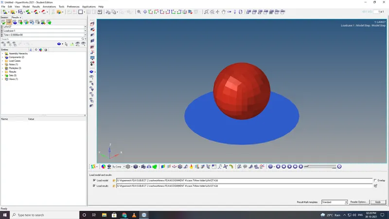
Given model - impact of the rigid ball on sheet metal for all these cases the material laws are changed for the sheet

Case 1 - Law 2 with EPS Max Failure and Failure Johnson card

Case 2 - Law 2 with EPS Max Failure and Ifail = 1,Dadv = 1 and Ixfem = 1(crack)

Case 3 - Law 2 with deleted fail johnson card

Case 4 - Law 2 with deleted Fail johnson and EPS Max Failure

Case 5 - Law 1 with density,E,nu

Case 6 - Law 27 with Eps based failure

Case 7 - Law 36 with straim rates curve

Case 1:

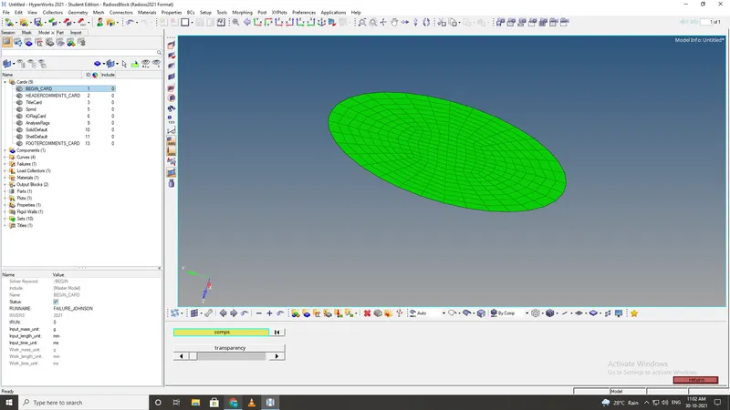
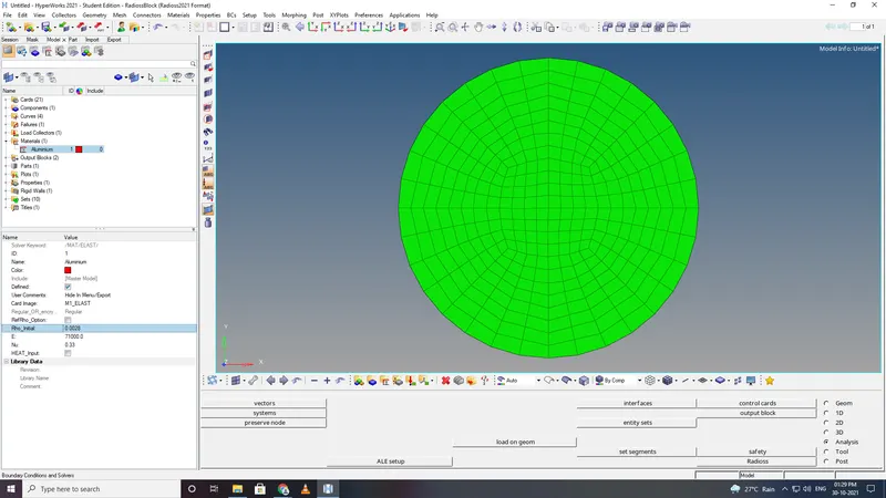
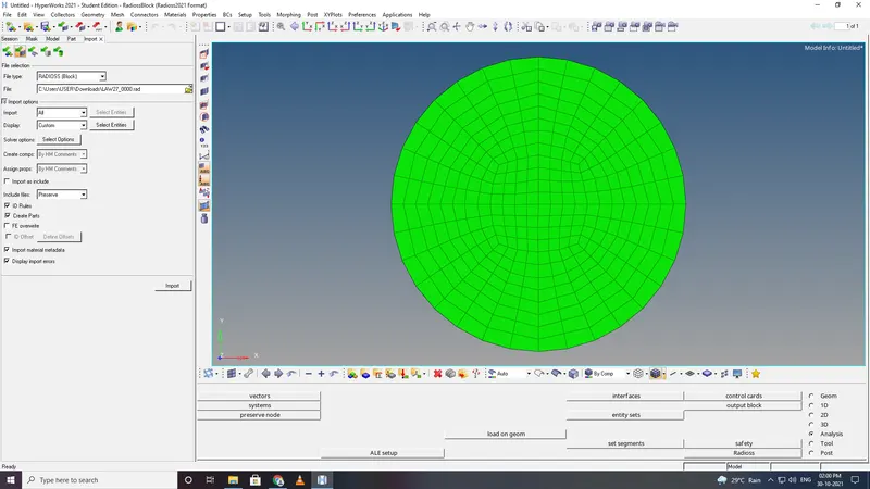
• Import the starter file into radios block
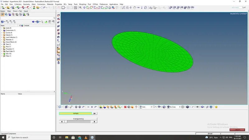
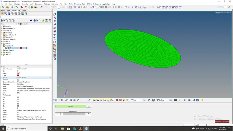
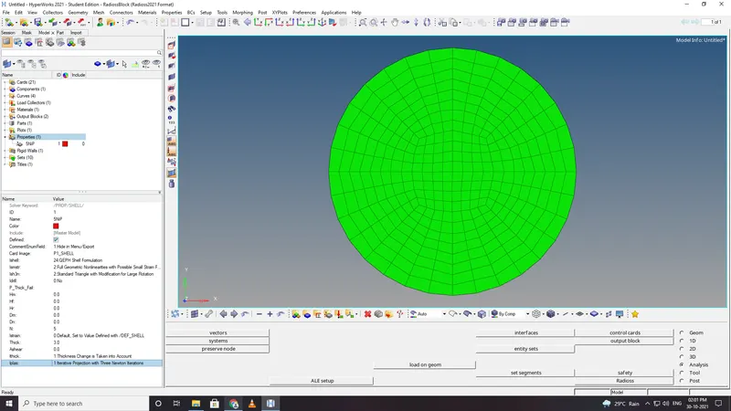
• Provide the shell properties to the components in this case the sheet metal
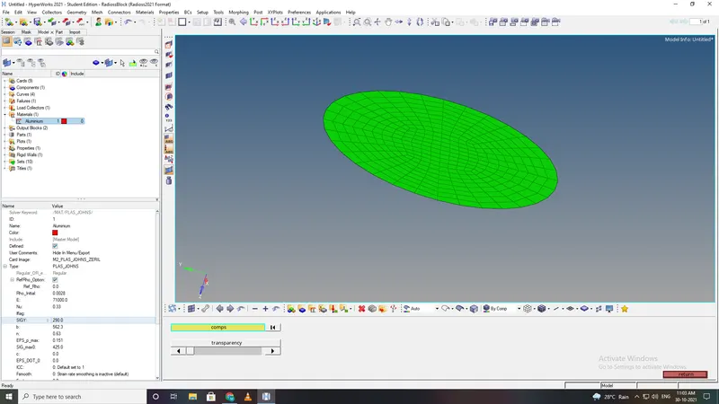
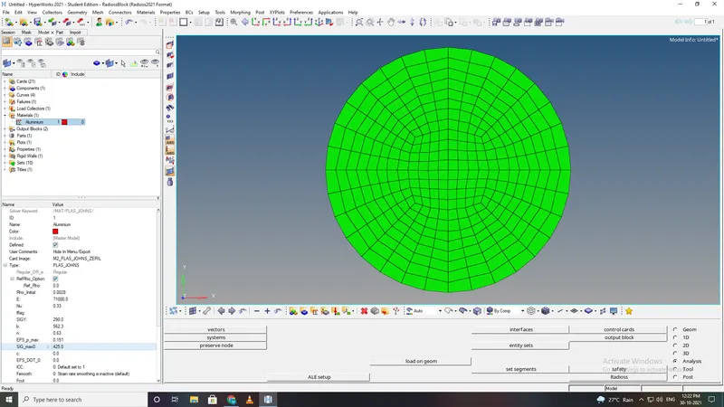
• Provide the material and failure to the component in this case Law 2 and failure jhonson card
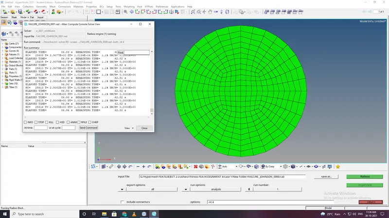
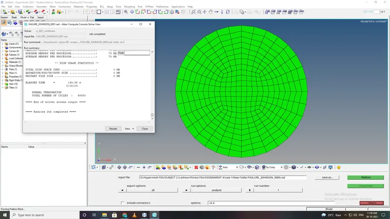
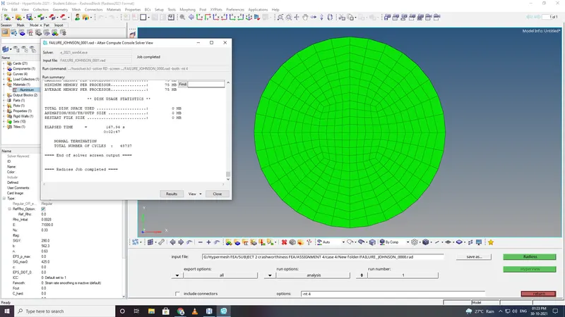
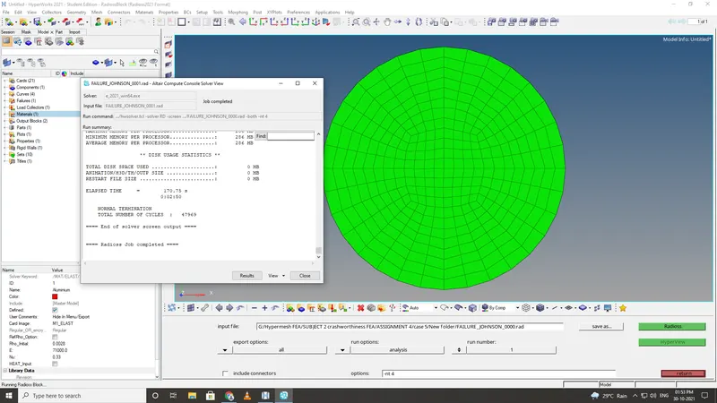
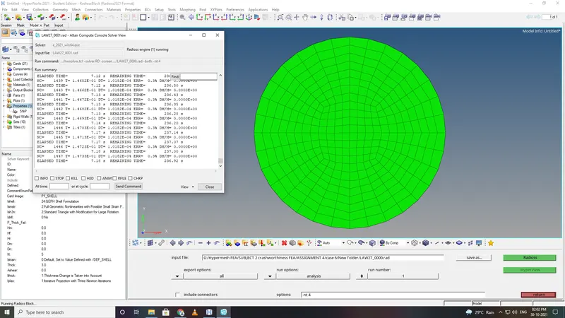
• Run radios and wait for the run to complete without any errors
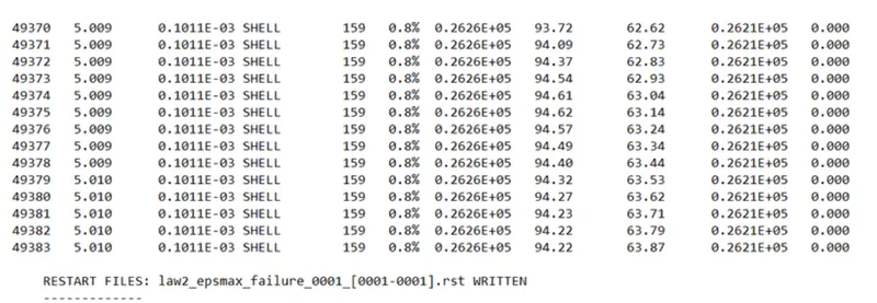
• Open the engine out file for energy error(should be less than 15%max) and mass errors(should be less than 1%)
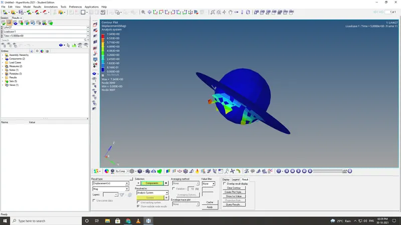
• open hyperview to obsever the animation and contour plots from H3d file.
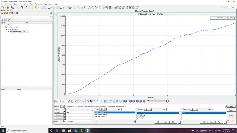
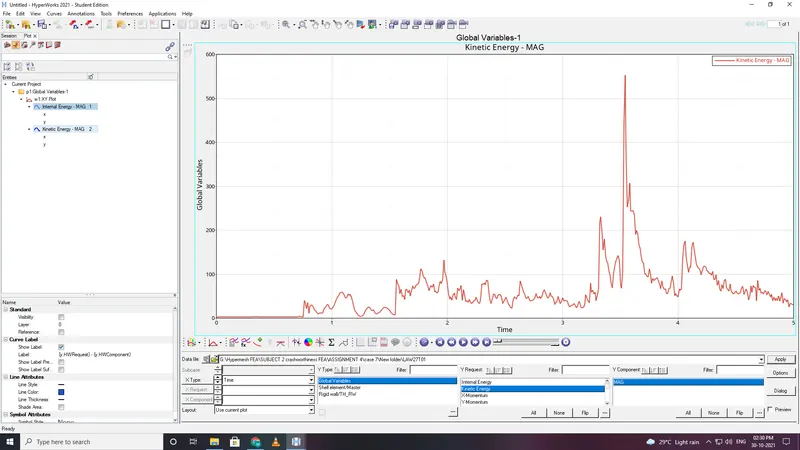
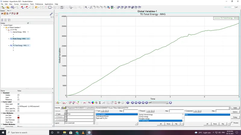
• open the hypergraphs 2d for observing the energy plot data from TA01 file.

• Run radios and wait for the run to complete without any errors

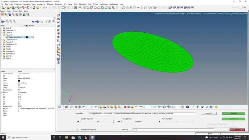
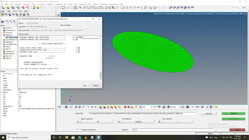
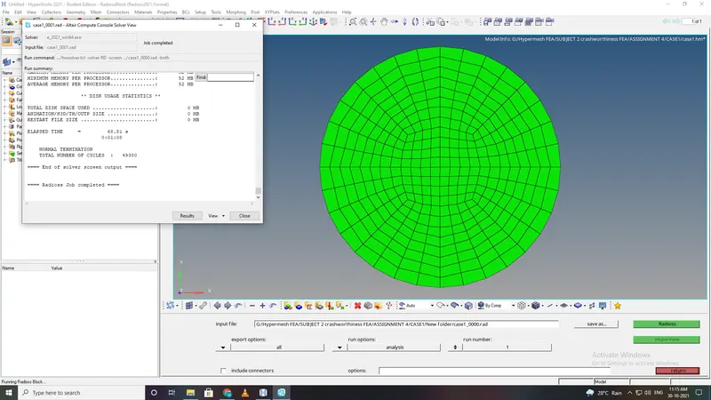
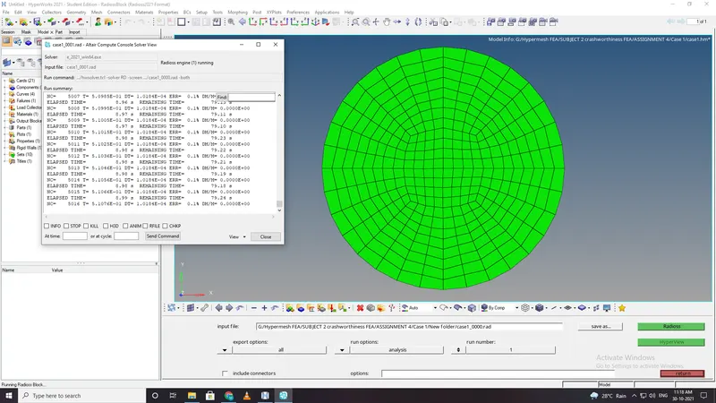
• This model represents the material stress as a function of plastic strain,strain rate and the temperature.
• In this case Ixfem = 0 so element is deleted is it reaches the rupture criteria.

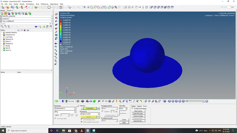
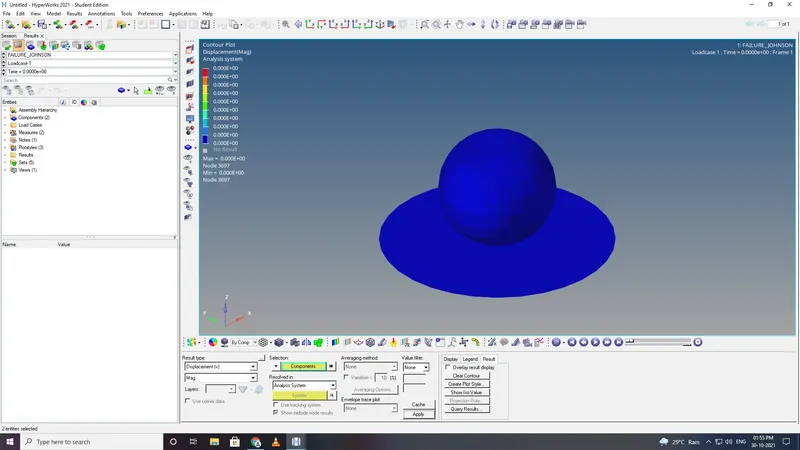
• open hyperview to obsever the animation and contour plots from H3d file.

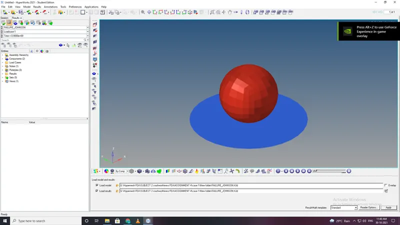
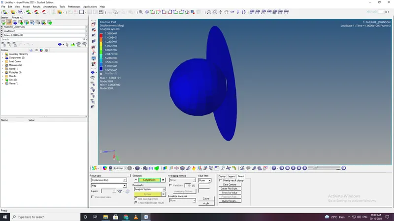
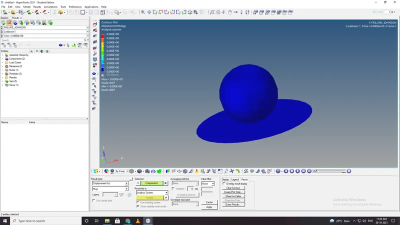
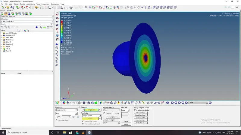
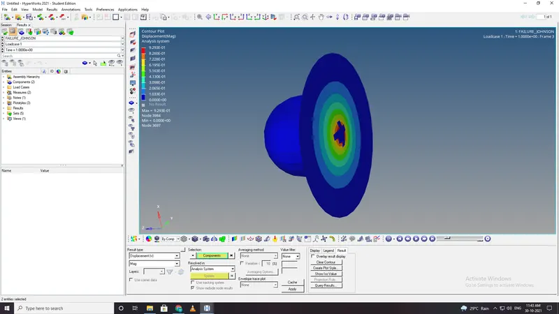
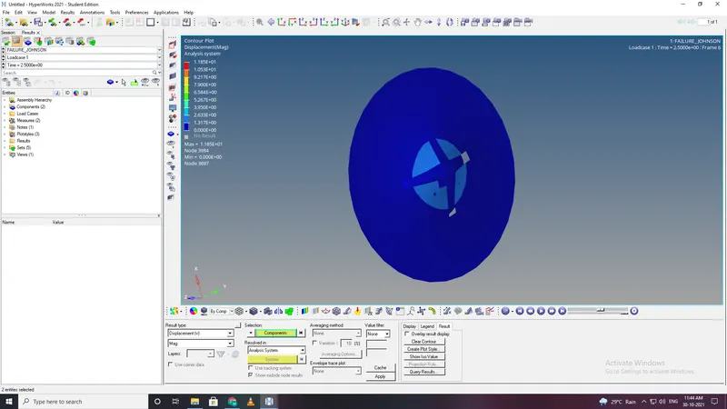
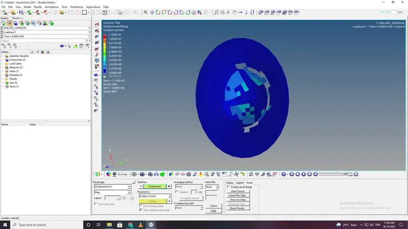
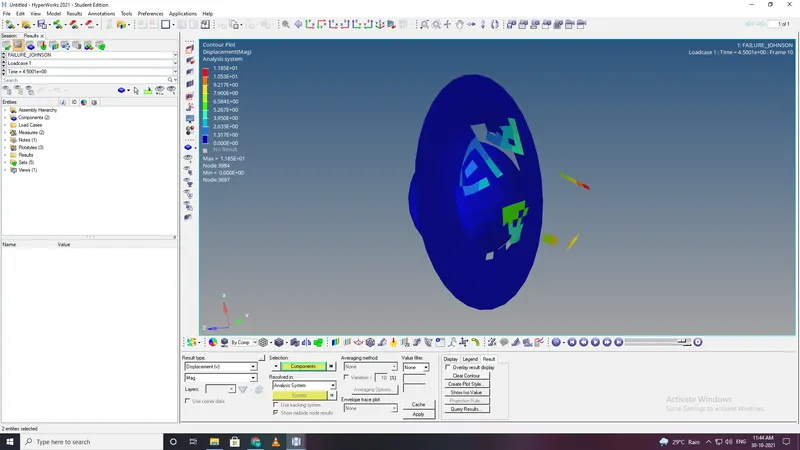
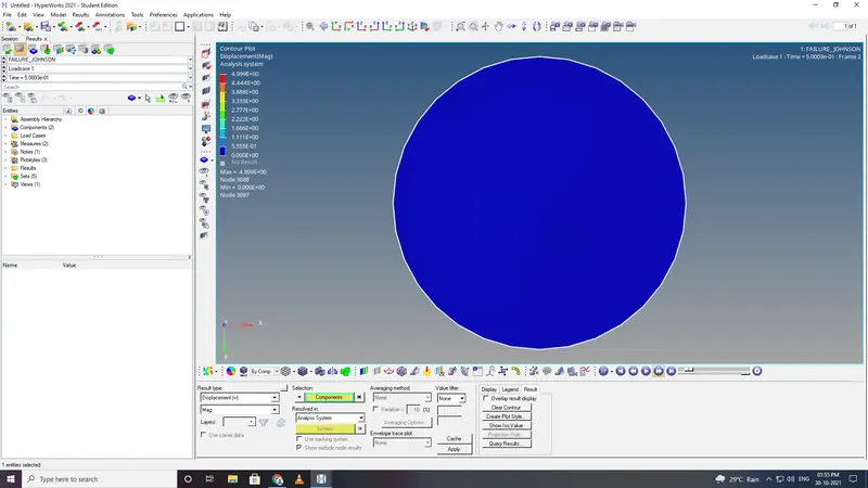
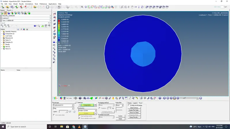
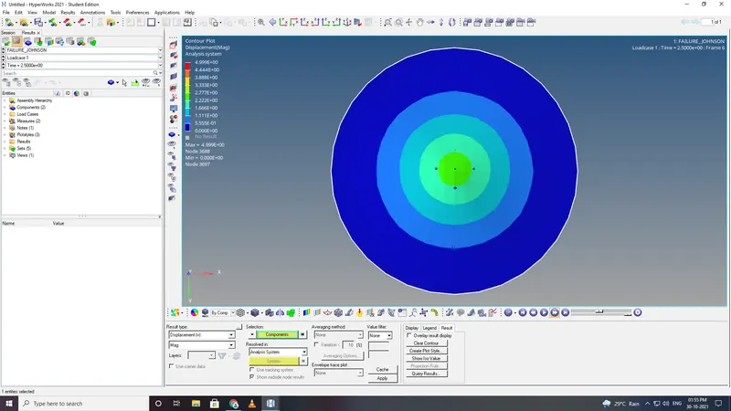
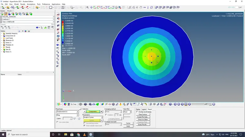
• We can observe the element are getting deleted as max plastic strain values are reached in the elements.But the crack propagation cannot be observed well as Ixfem is 0 in this case.

• open the hypergraphs 2d for observing the energy plot data from TA01 file.
• Energy error and mass error are within the limits- (less than 15% and 1% respectively) as the recommended shell properties are applied to the component

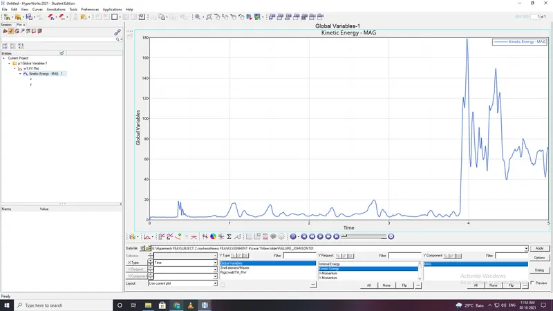
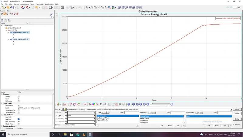
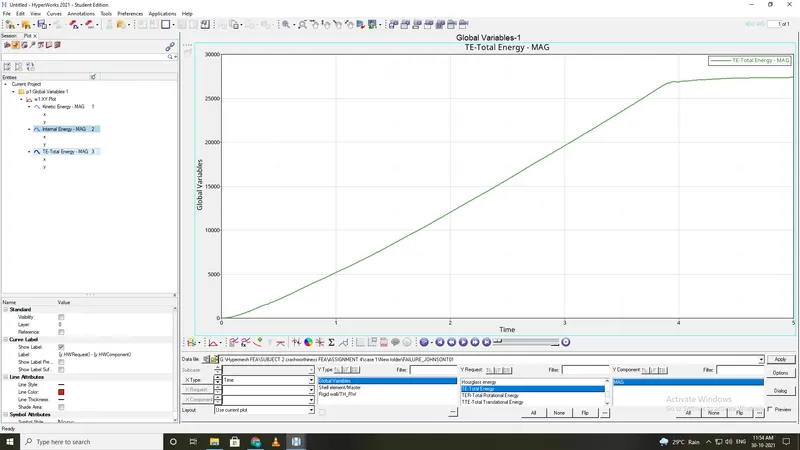
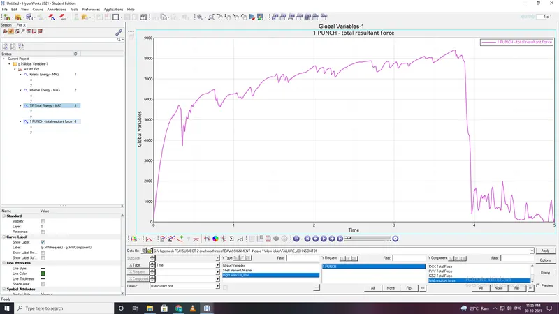
We can observe from the plots that the internal and total energy are reaches its peak value.

Case 2 :

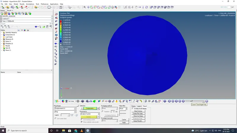
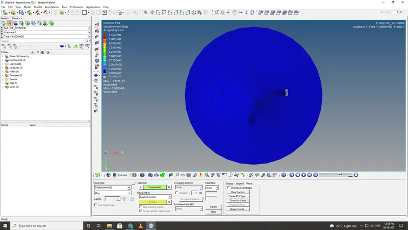
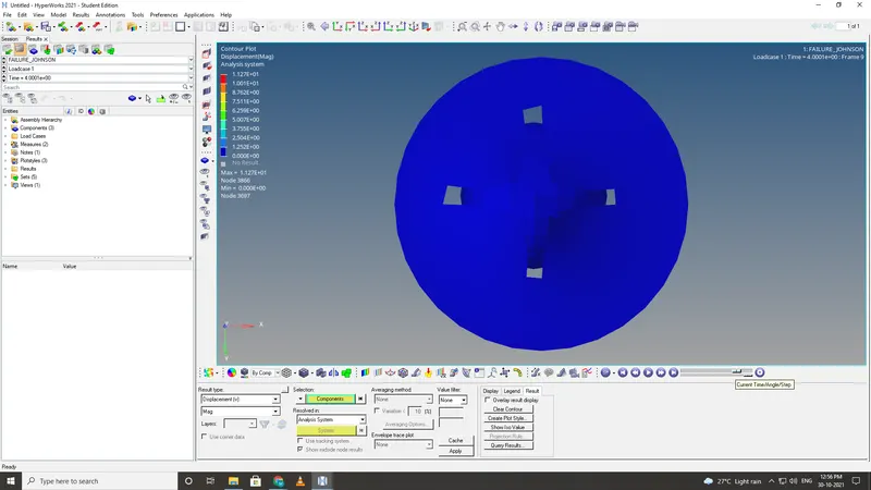
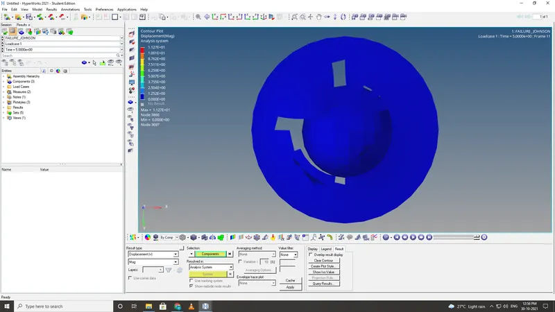
• In this same material is used except that in this case Ixfem= 1,so elements is cracked is it reaches the rupture criteria.
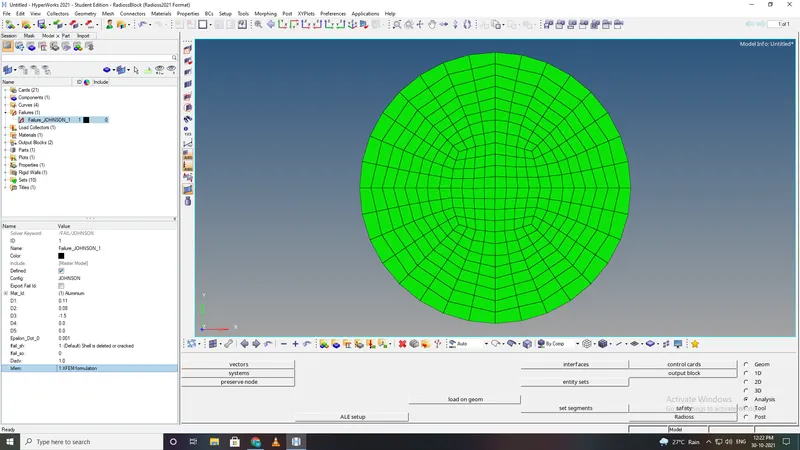
• Ifail_sh=1,shell failure flag of Ixfem=1,Dadv=1
• Run radios and wait for the run to complete without any errors
• Open the engine out file for energy error(should be less than 15%max) and mass errors(should be less than 1%).
• Animation and plot explantion
• Cumulative damage law based on the plastic strain accumalation is the failure model used here.
• open hyperview to obsever the animation and contour plots from H3d file.
• open the hypergraphs 2d for observing the energy plot data from TA01 file.
• Along with that Ixfem=1 hence crack propagation can be visible in this case before elements getting deleted.

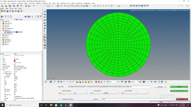
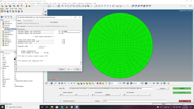
• Run radios and wait for the run to complete without any errors
• Open the engine out file for energy error(should be less than 15%max) and mass errors(should be less than 1%).

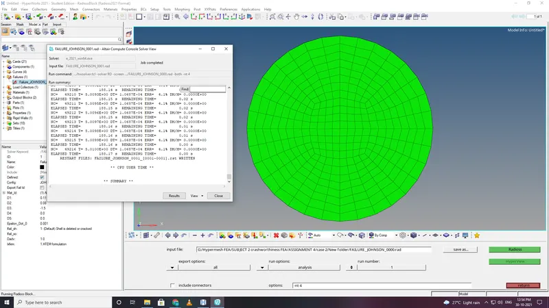
• open hyperview to obsever the animation and contour plots from H3d file.

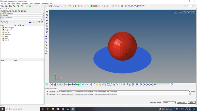
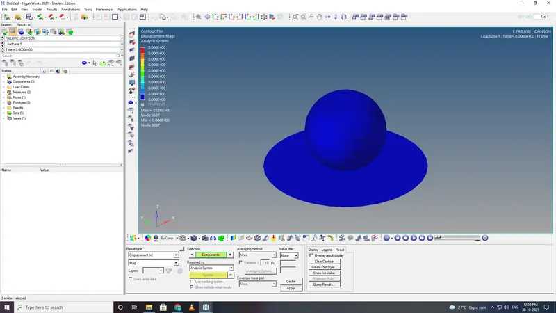
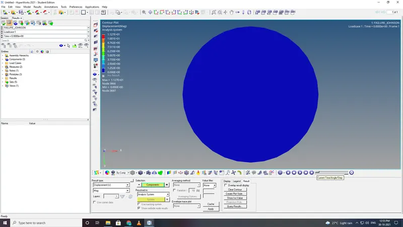
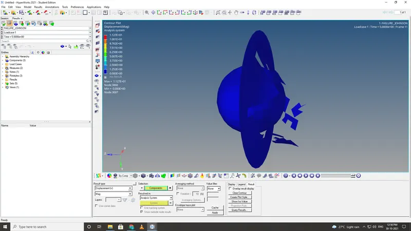
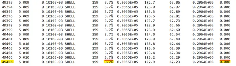• open the hypergraphs 2d for observing the energy plot data from TA01 file.

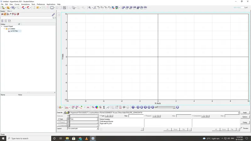
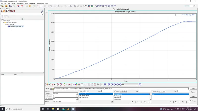
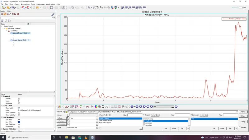
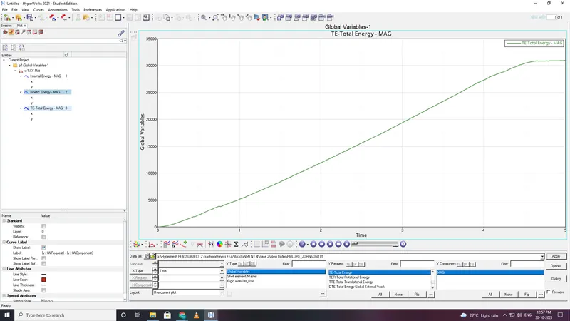
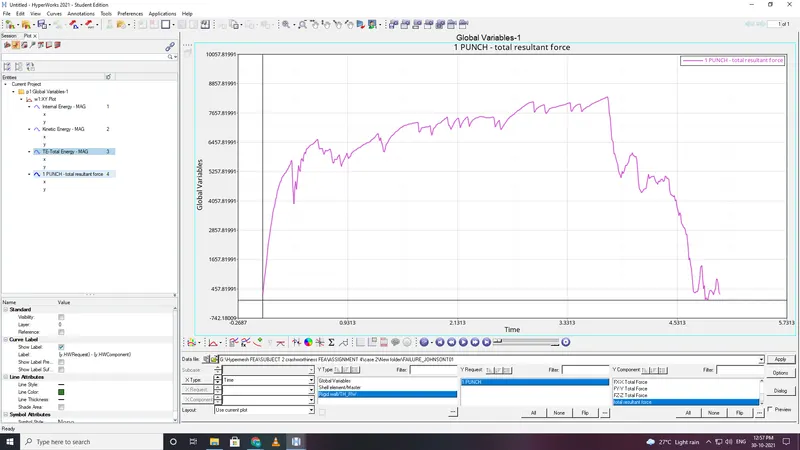
we can obseve from the above plots that around 4.5 ms which is later than the case 1 its because of the Ixfem and Dadv parameters which allows for deletion of elements only after crack propagation.

Case 3 :

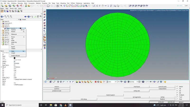
• same material but failure card is deleted.
• Eps max failure criteria is considered.Elements are deleted once
• when strain reaches the value of Eps max in one inetgration points,the corresponding shell elements is deleted.
• Run radios and wait for the run to complete without any errors
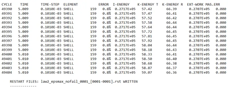
• Open the engine out file for energy error(should be less than 15%max) and mass errors(should be less than 1%).
• Animation and plots explations.
• open hyperview to obsever the animation and contour plots from H3d file.
• open the hypergraphs 2d for observing the energy plot data from TA01 file.
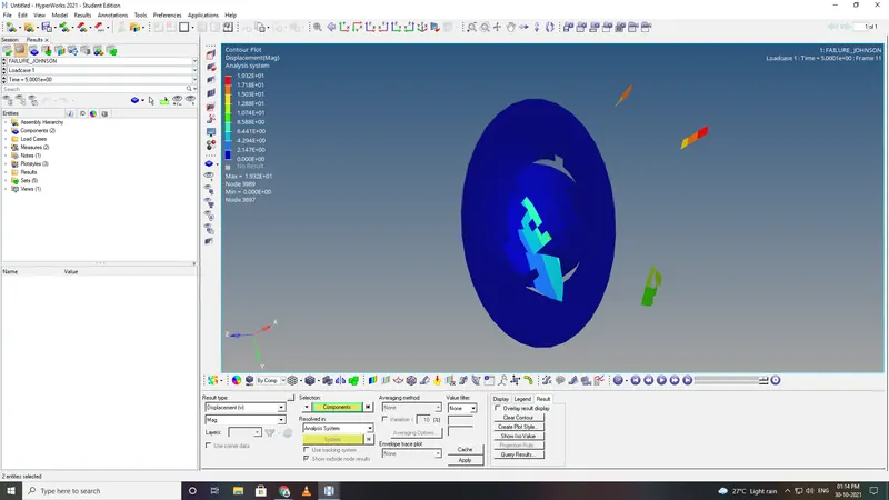
• From the annimation we observe that the elements are deleted the moment it reaches Eps max value as inputed.

• Run radios and wait for the run to complete without any errors
• Open the engine out file for energy error(should be less than 15%max) and mass errors(should be less than 1%).

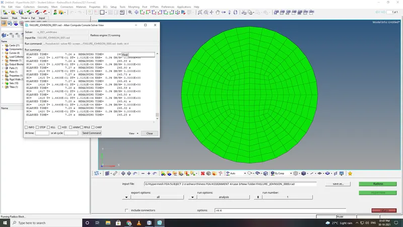
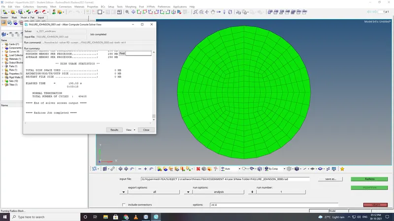
• open hyperview to obsever the animation and contour plots from H3d file.

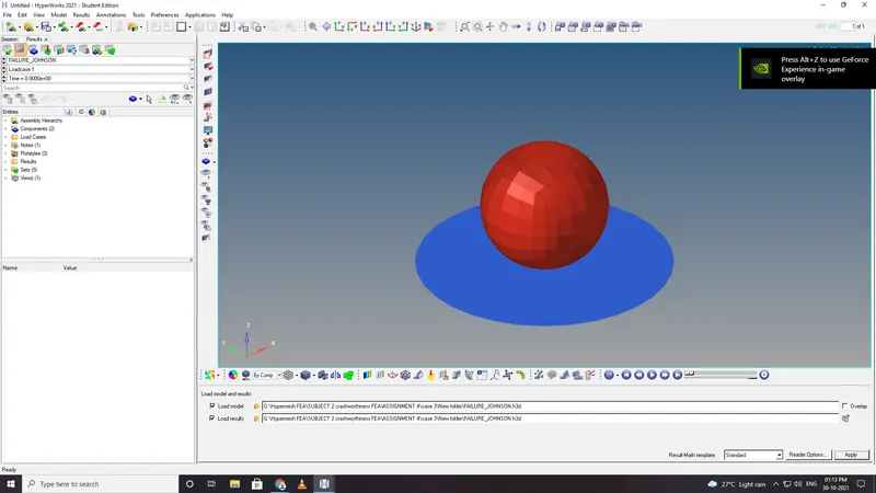
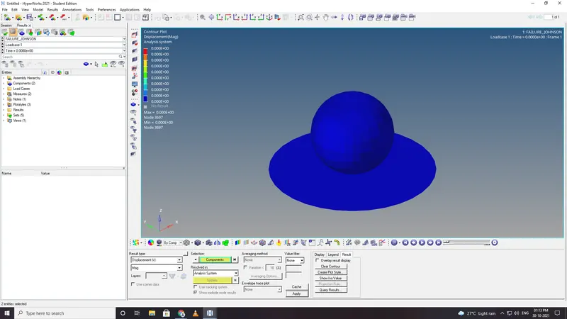
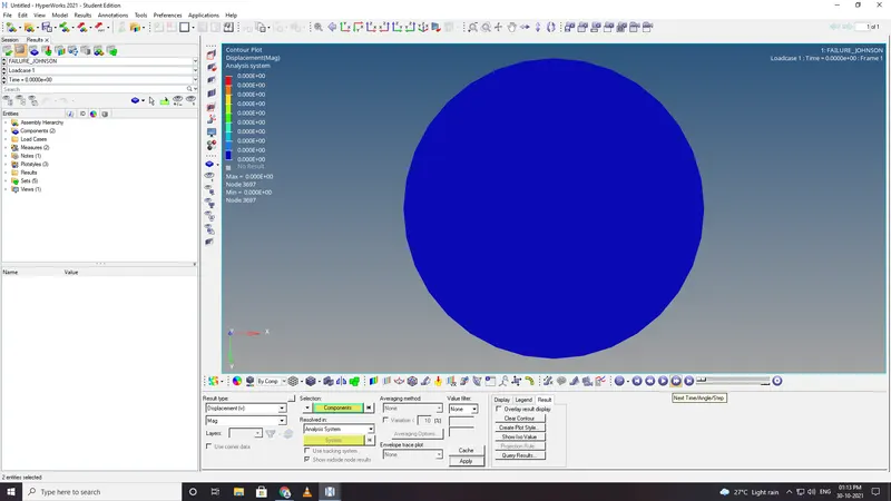
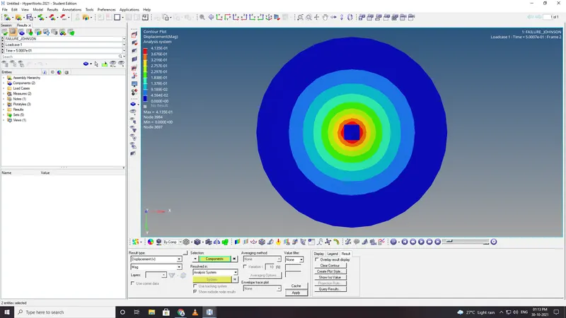
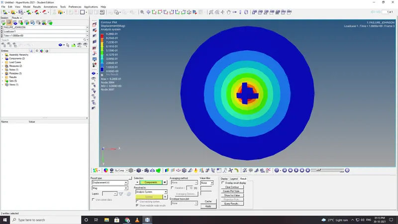
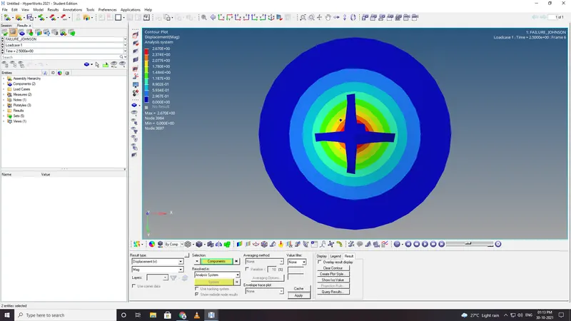
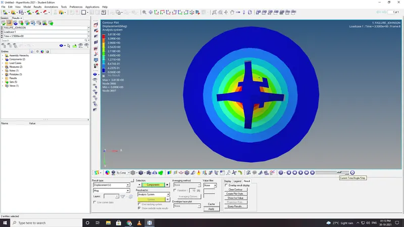
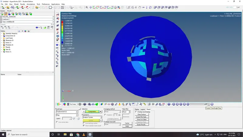
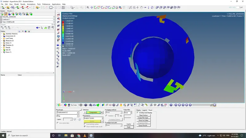
• open the hypergraphs 2d for observing the energy plot data from TA01 file.

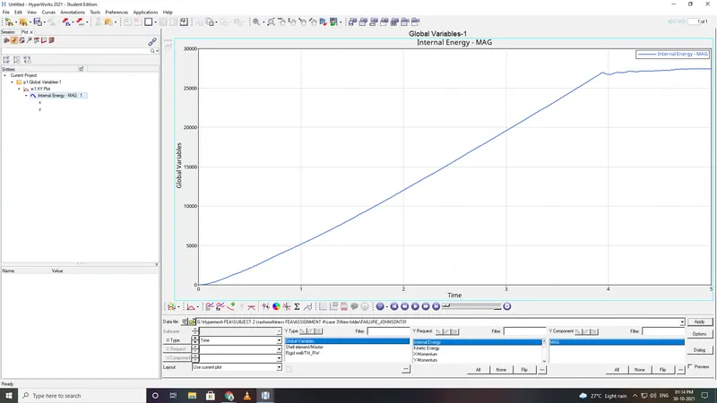
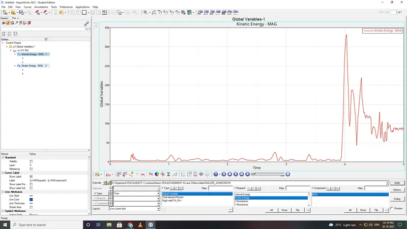
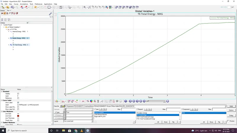
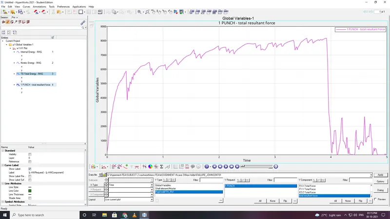
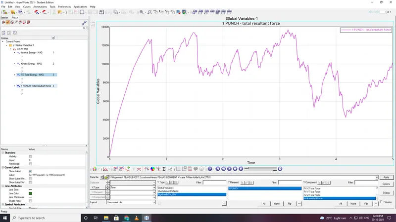
The plots are quite same in case 1. The impact of the ruputure due to the crack is not very noticable as compared to the case2,where total resultant forces were declining in a step manner.

Case 4:

• Same material but with failure johnson and eps max deleted.
• since the failure card is been deleted hence the solver sets Eps max is set to the value
• Run radios and wait for the run to complete without any errors
• Animation and plots explations.
• Now there is no failure criteria for the elements.
• Animation and plots explanation-elements are not getting deleted.failure criteria.
• open hyperview to obsever the animation and contour plots from H3d file.
• open the hypergraphs 2d for observing the energy plot data from TA01 file.

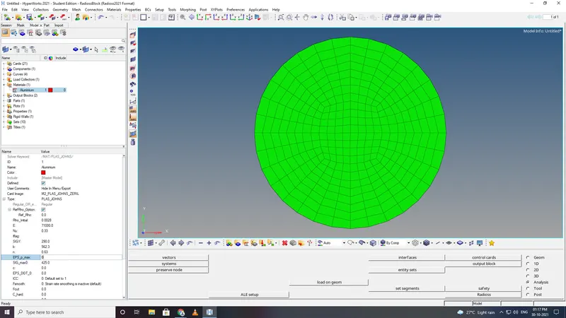
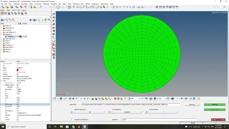
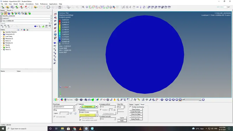
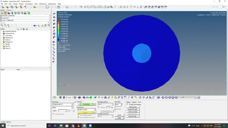
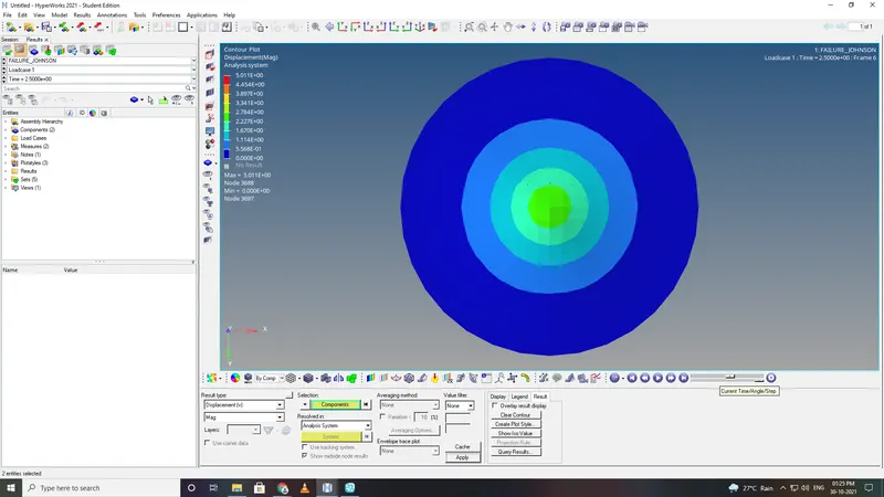
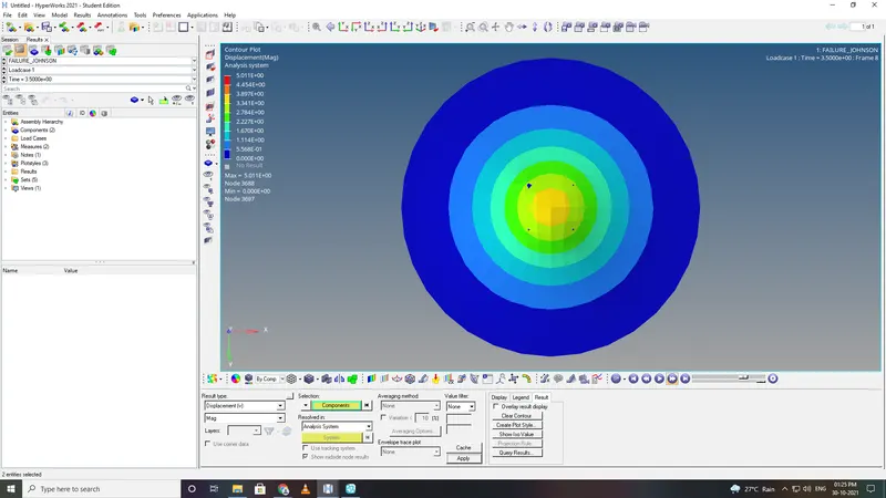
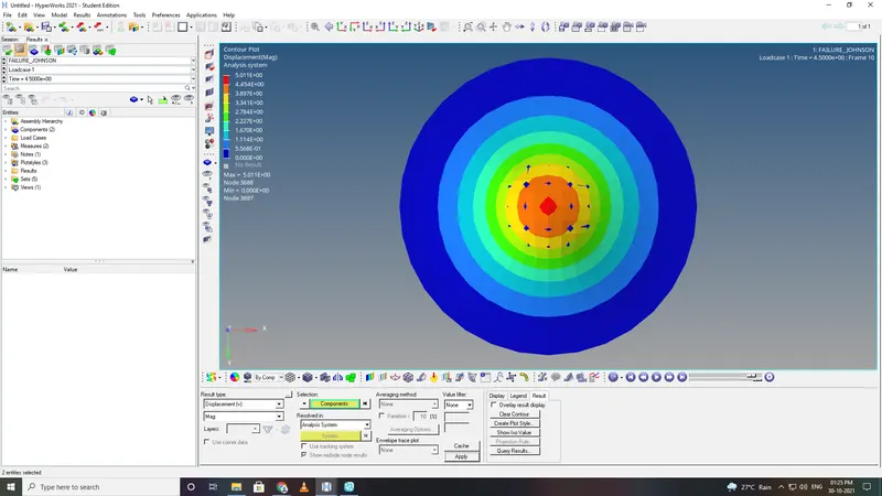
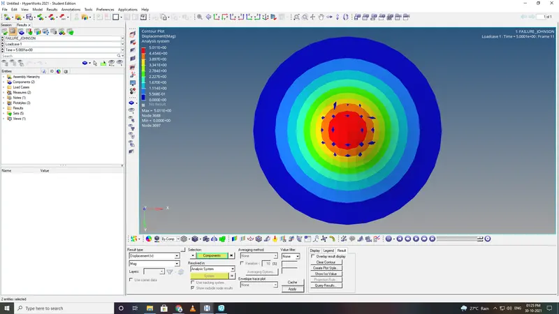
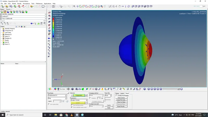
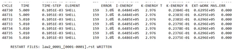
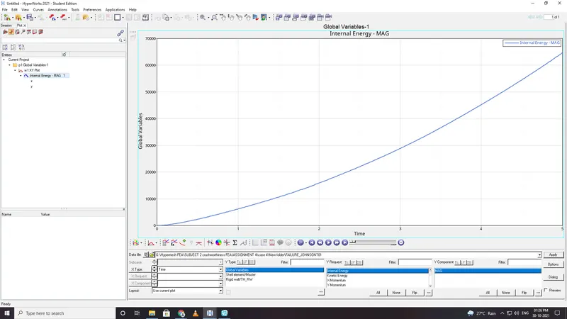
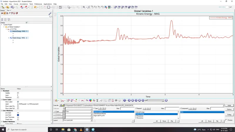
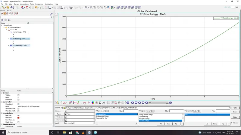
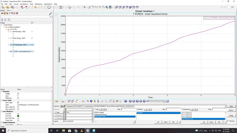
Energy plots and resultant forces can be similar to case 3.

Case 5 :

• In this case /MAT/LAW1 (ELAST)with density,E,nu is used.
• isotropic linear elastic material using Hooke's law.
• hence this law is used to model only elastic material.
• Run radios and wait for the run to complete without any error.
• Animation and plots explanation.elements are not getting deleted.
• Since we have selected a elastic material, behavior is very linear and there is no failure criteria for elements deletion.
• open hyperview to obsever the animation and contour plots from H3d file.
• open the hypergraphs 2d for observing the energy plot data from TA01 file.

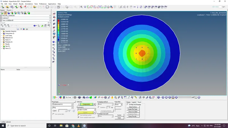
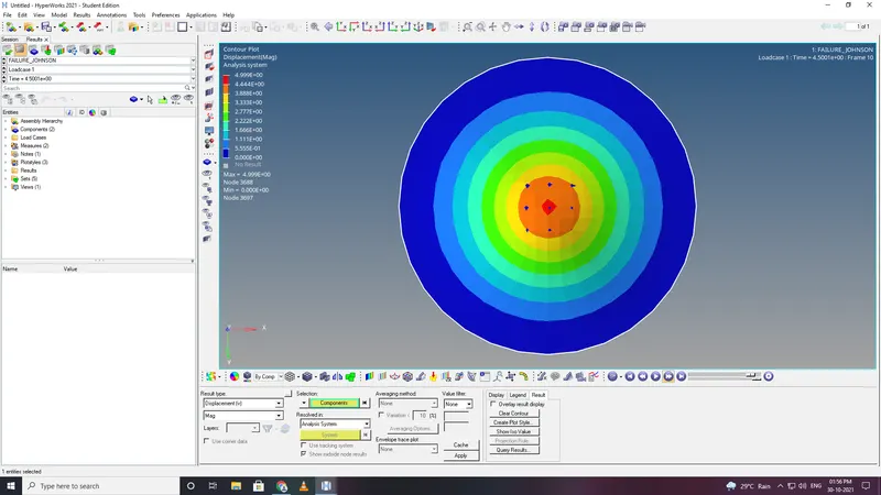
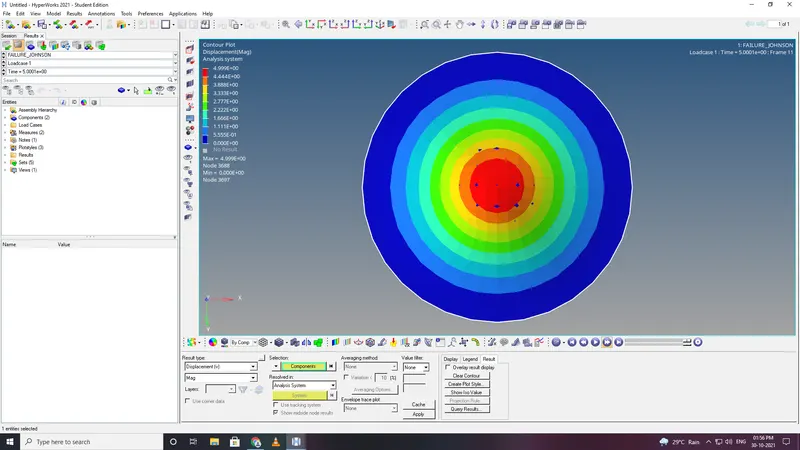
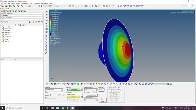
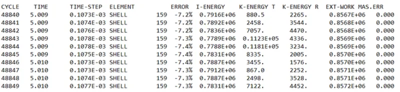
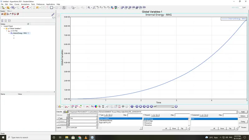
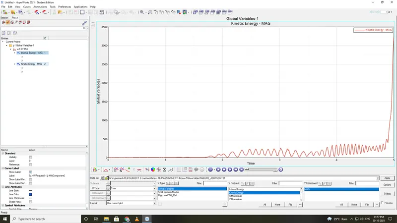
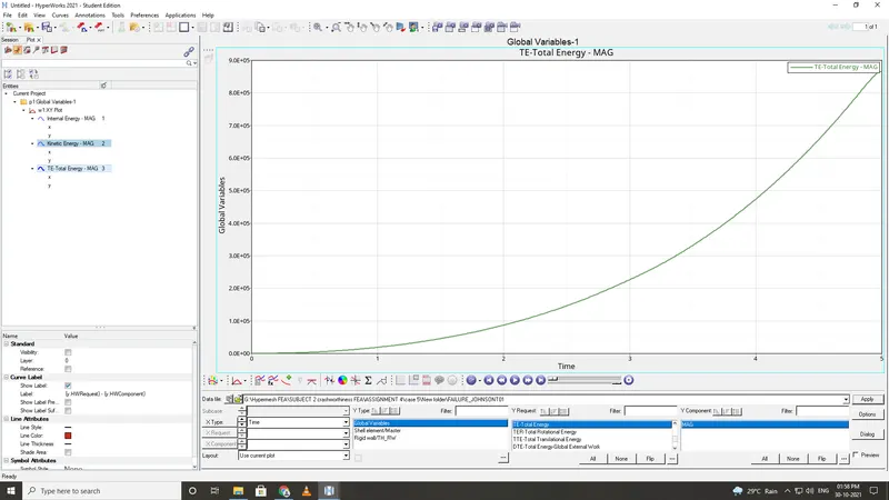
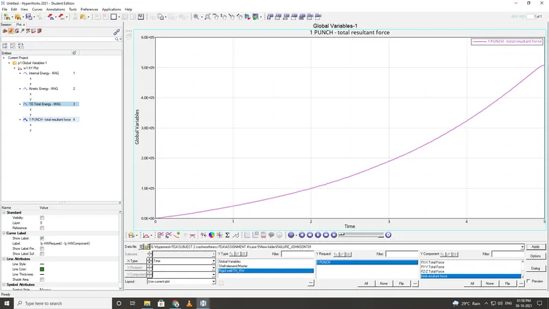
From the above plots we can see that internal energy and resultant forces on the rigid balls even higher than the case 4

There is no peaks or valleys in the resultant forces it goes linearly until the simulations time.

Case 6:

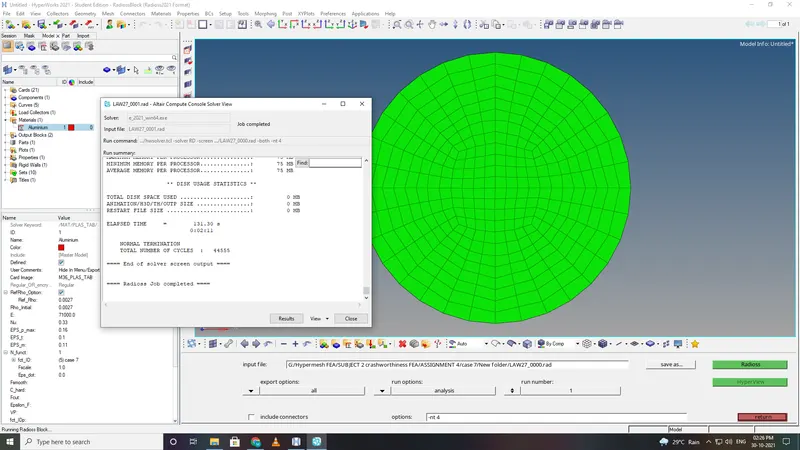
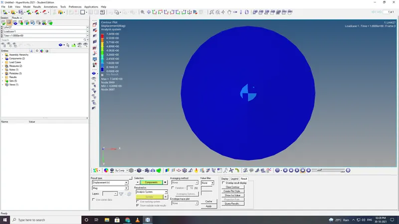
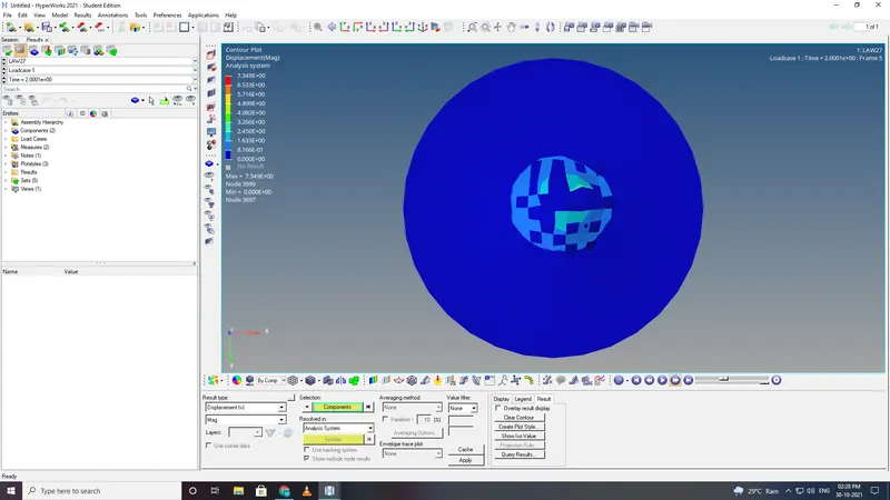
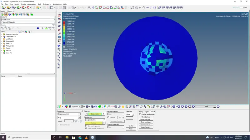
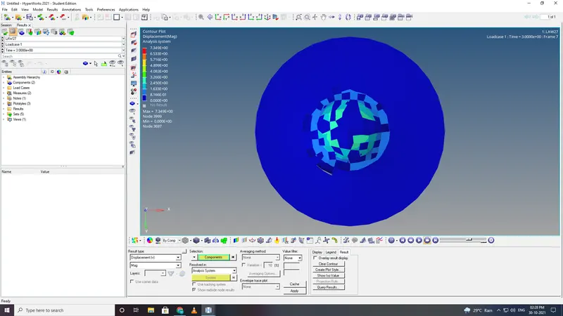
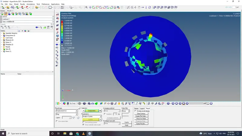
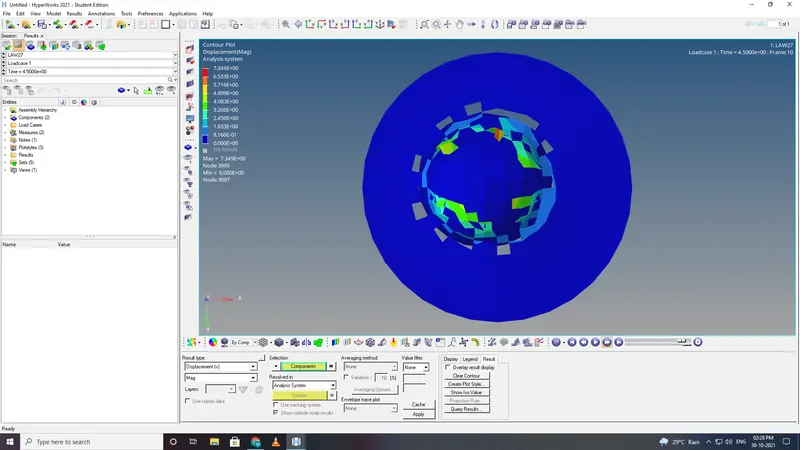
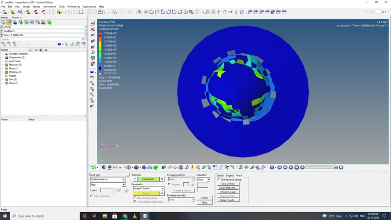
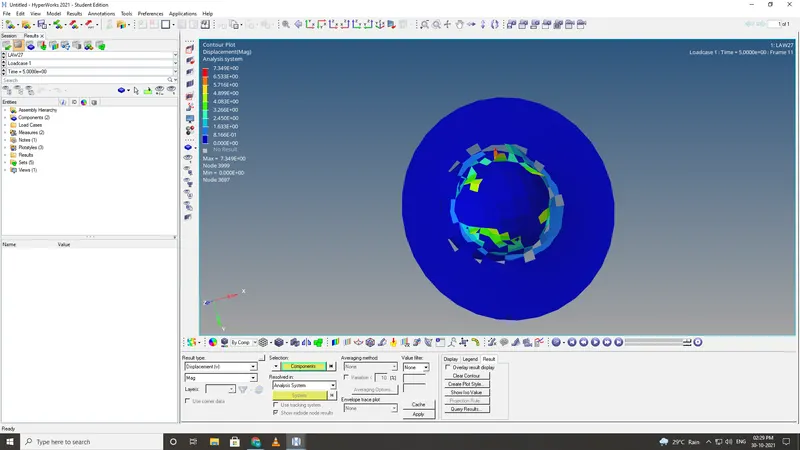
• In this case /MAT/LAW27 (PLAS_BRIT)is used. This law combaines an isotropic elasto_plastic johnson_cook material model.
• Run radios and wait for the run to complete without any error.
• In this model the material behaves as Linear elastic material.when the equivalent stress is lower than the plastic yield stress.
• For higher stress valus, the material behavior is plastic and the stress is calculated.
• once the max tensile strain is reached corresponding elements are deleted.
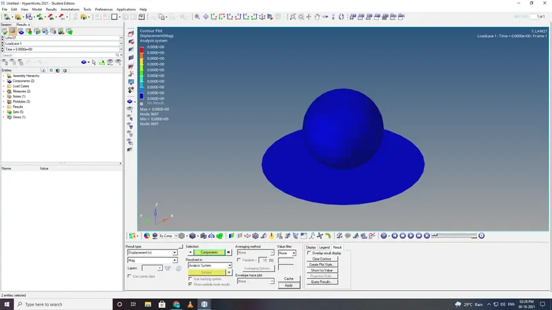
• open hyperview to obsever the animation and contour plots from H3d file.
• open the hypergraphs 2d for observing the energy plot data from TA01 file.

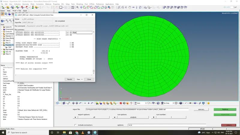
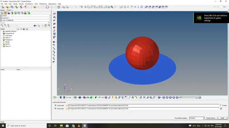
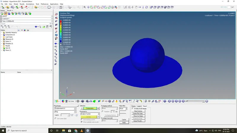
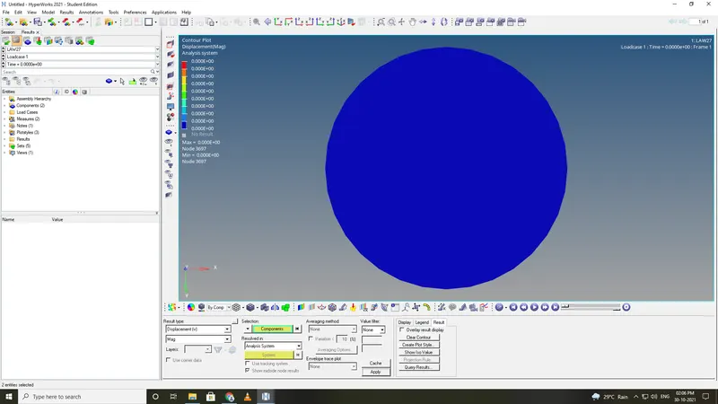
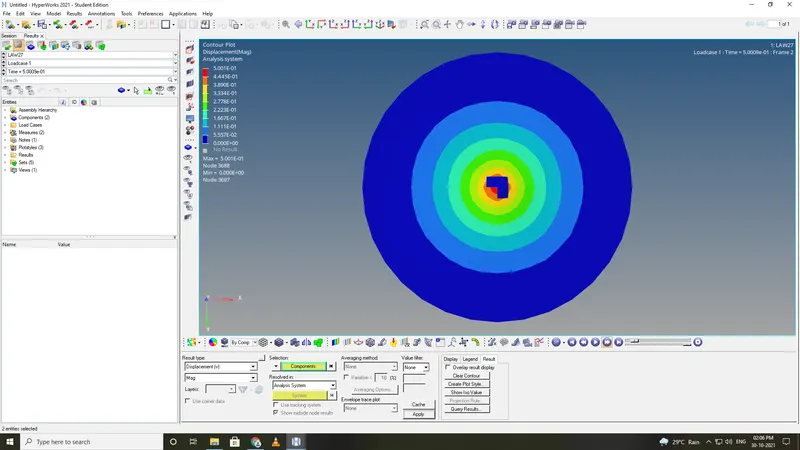
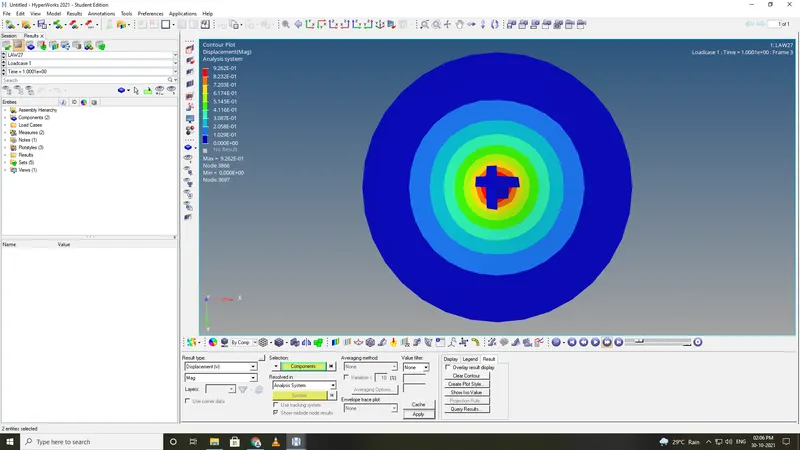
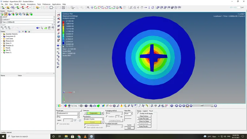
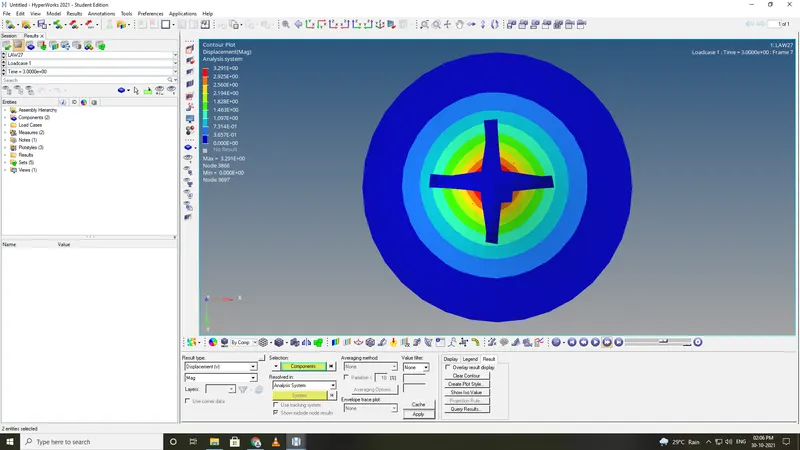
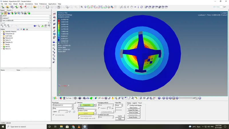
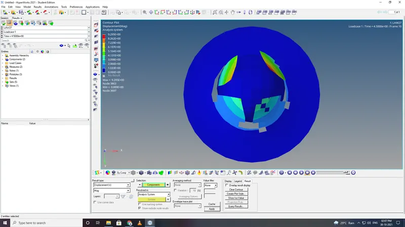
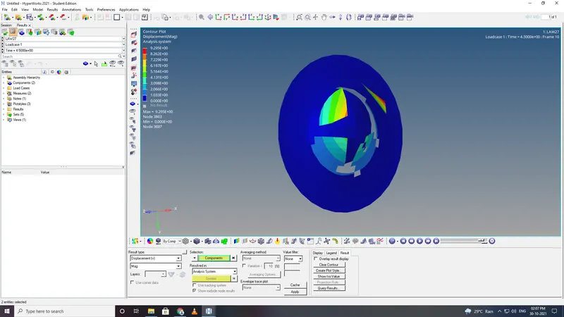
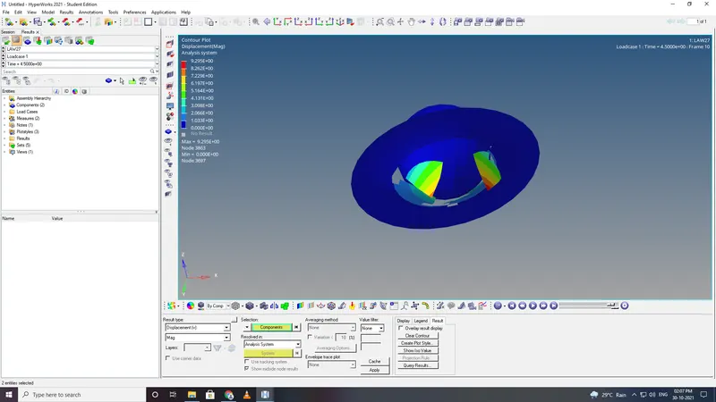
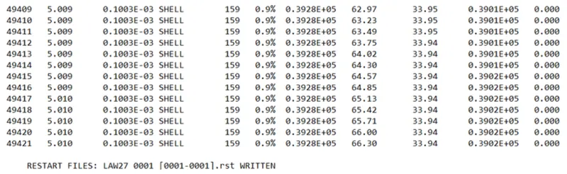
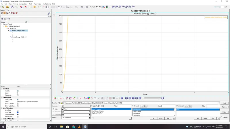
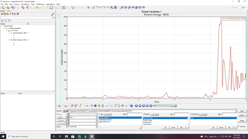
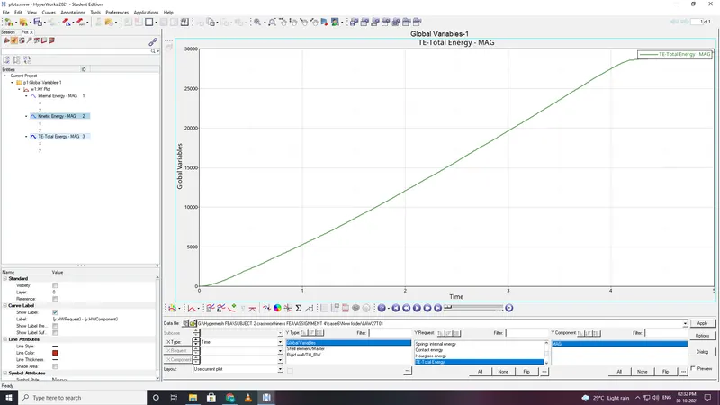
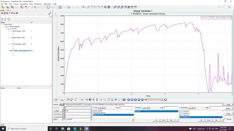
The sheet breaks into two parts showing its brittle nature. In terms of IE its reaches a peak value even after than we can see the rise in IE its due to the dissipation of strain energy from stressed elements.

Elements are deleted once the failure criteria is reached.

Case 7:

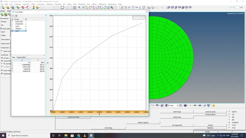
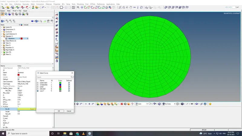
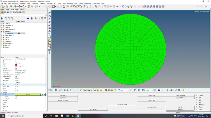
• In this case /MAT/LAW36 (PLAS_TAB)is used. This law models an elasto-plastic material using user_defined func.
• since the crashes happen within 120ms strain rates are very high so using this law user can input curves of true plastic strain vs stress for different rates into the model.
• it can be used for all types of elements shell or bricks.
• Stress strain curves inputted should not intersect and for cases where the stress strain rates are not inputted interpolation is done by solver for those cases.
• open hyperview to obsever the animation and contour plots from H3d file.
• open the hypergraphs 2d for observing the energy plot data from TA01 file.

CONCLUSION AND RESULTS:

	Cycles	Energy error	Mass error	Simulation time
Case 1	49384	1.2%	0	99.85 s
Case 2	49407	2.5%	0	114.89 s
Case 3	49405	1.2%	0	120.17 s
Case 4	48737	3.0%	0	121.19 s
Case 5	47969	4.0%	0	113.38 s
Case 6	49356	1.2%	0	117.88 s
Case 7	52204	-1.5%	0	128.50 s

• Hourglass energy remained almost Zero during all the cases.
• Mass error and energy error also were with limits due to the recommeded shell formulation.
• Case 1 and Case 6 are more realistic on field
• Case 2 with its crack propagation features would be usefull in small crak observation.
• Case 7 would be really usefull for simulating.if the teast data is available for different strain rates - would helps in crash based analysis giving more realistic results.