Week 3 - Solving second order ODEs

AIM : To write a program that solves the following ODE represents the equation of motion of a simple pendulum with damping.

• Simple pendulum consists of a mass m hanging from a string of length L and fixed at a point P. When displaced to an initial angle and released, the pendulum will swing back with periodic motion. With being the natural frequency of the motion
• The simple pendulum problem can be solved by using the second order ode functions and by solving these we will get the theta1 an theta2 values of the simple pendulum.

MATHEMATICAL EQUATION :

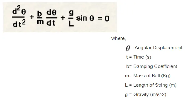
This equation is 2nd oder equation. Reason is d^2theta/dt^2 is a exponential form of 2.

substituting θ = θ1

dθ/dt = dθ1/dt = θ2--------------(1)

d^2θ/dt^2 = d^2θ1/dt^2 =d/dt (dθ1/dt) =d/dt (θ2)------------(2)

d^2θ1/dt^2+b/m dθ1/dt + g/l sinθ1 = 0

d/dt (θ2) + b/m θ2 + g/l sinθ1 = 0---------------------(3)

so from (1) & (3)

dθ1/dt = θ2 & d/dt (θ2) = -b/m θ2 - g/l sinθ1

d/dt[θ1;θ2] = [θ2;-b/m θ2 - g/l sinθ1]-------------------------(4)

EXPLANATION :

L=1 metre,

m=1 kg,

b=0.05.

g=9.81 m/s2. These values are inputed.

Simulate the motion between 0-20 sec, for angular displacement=0,angular velocity=3 rad/sec at time t=0.

initial condition for angular displacement=0,angular velocity=3.

tspan is the vector defining the beginning and end limits of integration.

t_span starting value 0 and ending value 10 and want to take 500 time steps.

t_span = linspace(0,10,500).

The function can be provided in the form of an anonymous function.

[t,result] = ode45(@(t,theta)ode_func(t,theta,b,g,l,m),t_span,theta_0).

Matlab’s standard solver for ordinary differential equations (ODEs) is the function
ode45. This function implements a Runge-Kutta method with a variable time step for
efficient computation

• The function ode45 takes 3 inputs.
• The 3 inputs are the function to be integrated.
• The time span and the initial conditions.
• ode45 is inbuilt solvering matlab.
• ode_func is define the function of input parameters.
• Input parameters are (t,theta,b,g,l,m).

code: 1

function [dtheta_dt] = ode_func(t,theta,b,g,l,m)
theta1 = theta(1)
theta2 = theta(2)
dtheta1_dt = theta2
dtheta2_dt = -(b/m)*theta2 - (g/l)*sin(theta1);
dtheta_dt = [dtheta1_dt;dtheta2_dt];
end

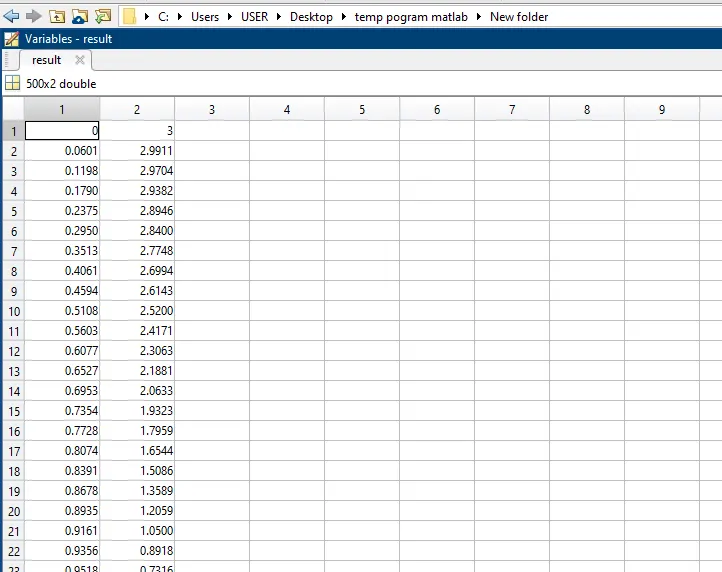
since solving ODE is results will be in column vector specified as 2 column.

• 1st column represents the angular displacement.
• 2nd column represents the angular velocity.

plotting

plot(t,result(:,1))

that is plot t,result from the beginning to the end in the 1st column.That represents the angular displacement.hold on
plot(t,result(:,2))

plot t,result from the beginning to the end in the 2nd column.That represents the angular velocity.
xlabel('time')
ylabel('plot')
legend('angular displacement','angular velocity')
hold off .

use for loop to run the code for different angular displacement

• for i=1:length(t).'length(t)' it means number of values in t that is 500 values. The value of 'i' is going to change from 1 value to 500 values. Each and every time it stores only one value.
• so the length of is assigned as 1m.
• co-ordinates of the base x0=0 & y0=0.
• co-ordinates of the ending points x1 = l*sin(result(i,1)) & y1 = -l*cos(result(i,1).

plotting the string of the pendulum.

plot [x base x end],[y base y end] with color of red. which is plot([x0 x1],[y0 y1],'color','r').

hold on.

plotting horizontal base line of pendulum.

plot([1 -1],[0 0],'color','b').

plotting pendulum ball.

plot(x1,y1,'.','markersize',50)

Before the 'for loop' .counter ct = 1 is added. After plotting the x co-ordinte & y co-ordinate the axis is assigned as ([-1 1 -1 1]).

hold off.

M(ct)= getframe(gcf) is added . That is to get a individual frames and save is in array called M(ct). (ct) represents each and every frames that will get a frame .(gcf) is nothing but the current frame in the figure window. After thar the counter ct = ct+1 incrementing is added and give the end.

CODE : 2

clear all
close all
clc


b = 0.05
g = 9.81
l = 1
m = 1

%initial condition
theta_0=[0;3];

%time points
t_span = linspace(0,10,500);

%solve one
[t,result] = ode45(@(t,theta)ode_func(t,theta,b,g,l,m),t_span,theta_0);


plot(t,result(:,1))
hold on
plot(t,result(:,2))
xlabel('time')
ylabel('plot')
legend('angular displacement','angular velocity')
hold off
ct=1;
for i=1:length(t)
x0 = 0
y0 = 0
x1 = l*sin(result(i,1));
y1 = -l*cos(result(i,1));

figure(2)
%string of the pendulum
plot([x0 x1],[y0 y1],'color','r')
hold on
%horizontal base line of pendulum
plot([1 -1],[0 0],'color','b')
%pendulum ball
plot(x1,y1,'.','markersize',50)
axis([-1 1 -1 1])
hold off

M(ct)= getframe(gcf);
ct = ct+1
end

moviein(M)
videofile = VideoWriter('pendulum_ode.avi','uncompressed AVI');
open(videofile)
writeVideo(videofile,M)
close(videofile)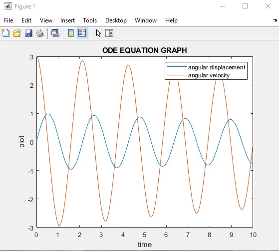

THE ANIMATION OF SIMPLE PENDULUM

ERROR :

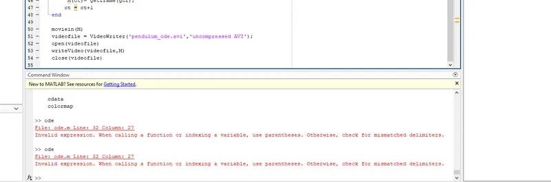
x1 = l*sin(result(i,1). the close bracket has missing.x1 = l*sin(result(i,1)).

REFFERENCE :

https://in.mathworks.com/help/matlab/ref/ode45.html.

https://in.mathworks.com/help/matlab/creating_plots/create-line-plot-with-markers.html.

CONSULTION :

A simulation of simple pendulum with damping was created using MATLAB program.