Week 4.1 - Genetic Algorithm

Classical Algorithm	Genetic Algorithm
Generates a single point at each iteration. The sequence of points approaches an optimal solution.	Generates a population of points at each iteration. The best point in the population approaches an optimal solution.
Selects the next point in the sequence by a deterministic computation.	Selects the next population by computation which uses random number generators.

GA is uses 3 types

• selection rule
• crossover rule
• mutation rule

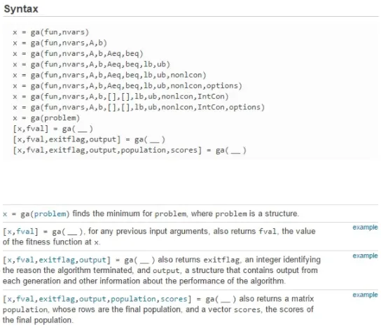
SYNTAX :

Stalagmite function :

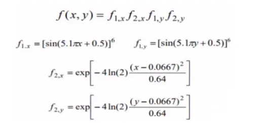
• These formula & equations are represents the stalagmite function.
• Intial stalagmite function is defined.

function [F] = stalagmite(input_vector) %stalagmite function with input as input_vetor which cotains x and y variables.
x=input_vector(1);
y=input_vector(2);

f1_x = (sin(5.1*pi*x+0.5)).^6;
f1_y = (sin(5.1*pi*y+0.5)).^6;

f2_x = exp(-4*log(2)*((x-0.0667).^2)/0.64);

f2_y = exp(-4*log(2)*((y-0.0667).^2)/0.64);

[F] = -(f1_x.*f1_y.*f2_x.*f2_y) ;
end

• A negative sign is used for the fundtion to obtain maxima of the function.

There 3 cases

1. unbounded inputs.
2. bounded inputs.
3. bounded iputs with modifications of population size.

1st iteration :

To find the global maxima

clear all
close all
clc
  
%defining our search space
x = linspace(0,0.6,150);
y = linspace(0,0.6,150);

%creating a 2dimensional mesh
[xx,yy] = meshgrid(x,y);

%evaluating the stalagmite function
for i =1:length(xx)
    for j =1:length(yy)
        input_vector(1) = xx(i,j);
        input_vector(2) = yy(i,j);
        f(i,j) = stalagmite(input_vector);
    end
end

surfc(xx,yy,f);
shading interp
    

tic 
%step 5
%study the statical behaviar
num_cases = 50; %number of iteration for which will evaluate the fitness
for i = 1:num_cases
    [inputs, fopt(i)] = ga(@stalagmite,2);
    xopt(i) = inputs(1);
    yopt(i) = inputs(2);
end
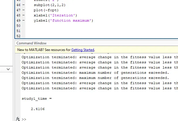
study1_time = toc
F = -f;
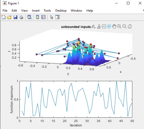
figure(1)
subplot(2,1,1)
hold on
surfc(x,y,F) %generating the surface
shading interp
plot3(xopt,yopt,-fopt,'marker','o','markersize',5,'markerfacecolor','r')
title('unbounded inputs')
xlabel('x')
ylabel('y')
zlabel('f')
subplot(2,1,2)
plot(-fopt)
xlabel('Iteration')
ylabel('function maximum')

step1 : Defining our search space. using linspace command. start from 0 value and end to 0.6 values.which has 150 values.
x = linspace(0,0.6,150);
y = linspace(0,0.6,150);
Creating a 2dimensional mesh using meshgrid command.
[xx,yy] = meshgrid(x,y);

• using the meshgrid command, row vector x and y converted into matrices xx and yy.

step 2: evaluating the stalagmite function using 'for loop'.
for i =1:length(xx)
for j =1:length(yy)
input_vector(1) = xx(i,j);
input_vector(2) = yy(i,j);
f(i,j) = stalagmite(input_vector);
end
end

• with the help of for loop the input vector are defined using the matrices pf xx and yy.

step 3 : study the statical behaviour.num of cases = 50. which is umber of iteration for which will evaluate the fitness. using 'for loop'.
for i = 1:num_cases
[inputs, fopt(i)] = ga(@stalagmite,2);
xopt(i) = inputs(1);
yopt(i) = inputs(2);
end

• the study is timed using tic toc command.

step 4 : ploting

plot3(xopt,yopt,-fopt,'marker','o','markersize',5,'markerfacecolor','r')
title('unbounded inputs')
xlabel('x')
ylabel('y')
zlabel('f')
subplot(2,1,2)
plot(-fopt)
xlabel('Iteration')
ylabel('function maximum')

• markers are done by plot3 command over the fitness values.

study1_time =

2.4106

2nd iteration :

In this 2nd iteration the lower and upper bounds are defined which is global maximas .

clear all
close all
clc
  
%defining our search space
x = linspace(0,0.6,150);
y = linspace(0,0.6,150);

%creating a 2dimensional mesh
[xx, yy] = meshgrid(x,y);

%evaluating the stalagmite function
for i = 1:length(xx)
    for j = 1:length(yy)
        input_vector(1) = xx(i,j);
        input_vector(2) = yy(i,j);
        f(i,j) = stalagmite(input_vector); %value of the function in given search space
    end
end
%study2 - statical behaviar of upper and lower bounds
tic
num_cases = 50;
for i = 1:num_cases
    [inputs,fopt(i)] = ga(@stalagmite,2,[],[],[],[],[0;0],[0.6;0.6]);% define a lower(0,0) and upper(0.6,0.6)
    xopt(i) = inputs(1);
    yopt(i) = inputs(2);
end
study2_time = toc
figure(2)
F = -f;
subplot(2,1,1)
hold on
surfc(x,y,F) %generating the surface
shading interp
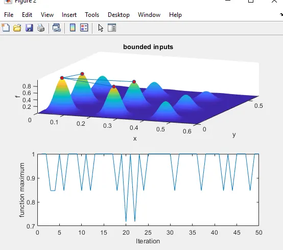
plot3(xopt,yopt,-fopt,'marker','o','markersize',5,'markerfacecolor','r')
title('bounded inputs')
xlabel('x')
ylabel('y')
zlabel('f')
subplot(2,1,2)
plot(-fopt)
xlabel('Iteration')
ylabel('function maximum')

step1 : Defining our search space. using linspace command. start from 0 value and end to 0.6 values.which has 150 values.
x = linspace(0,0.6,150);
y = linspace(0,0.6,150);
Creating a 2dimensional mesh using meshgrid command.
[xx,yy] = meshgrid(x,y);

• using the meshgrid command, row vector x and y converted into matrices xx and yy.

step 2: evaluating the stalagmite function using 'for loop'.
for i =1:length(xx)
for j =1:length(yy)
input_vector(1) = xx(i,j);
input_vector(2) = yy(i,j);
f(i,j) = stalagmite(input_vector);
end
end

• with the help of for loop the input vector are defined using the matrices pf xx and yy.

step 3 : statical behaviour of upper and lower bounds.
tic
num_cases = 50;
for i = 1:num_cases
[inputs,fopt(i)] = ga(@stalagmite,2,[],[],[],[],[0;0],[0.6;0.6]); define a lower(0,0) and upper(0.6,0.6)
xopt(i) = inputs(1);
yopt(i) = inputs(2);
end

step 4: to produce the contour plot of stalagmite function.

plot3(xopt,yopt,-fopt,'marker','o','markersize',5,'markerfacecolor','r')
title('bounded inputs')
xlabel('x')
ylabel('y')
zlabel('f')
subplot(2,1,2)
plot(-fopt)
xlabel('Iteration')
ylabel('function maximum')

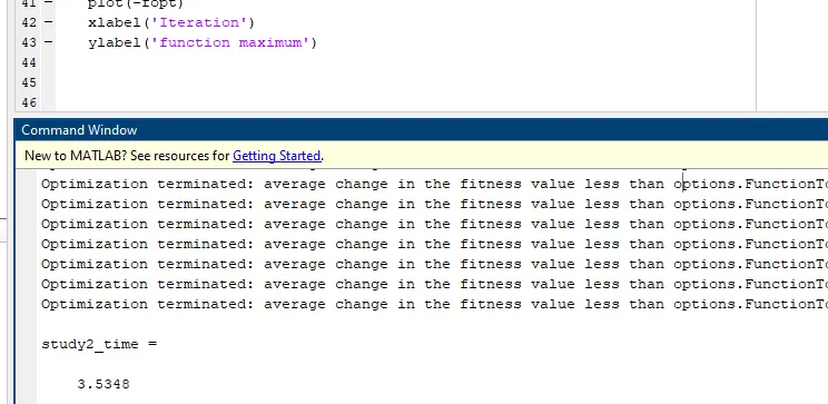
study2_time =

3.5348

3rd iteration :

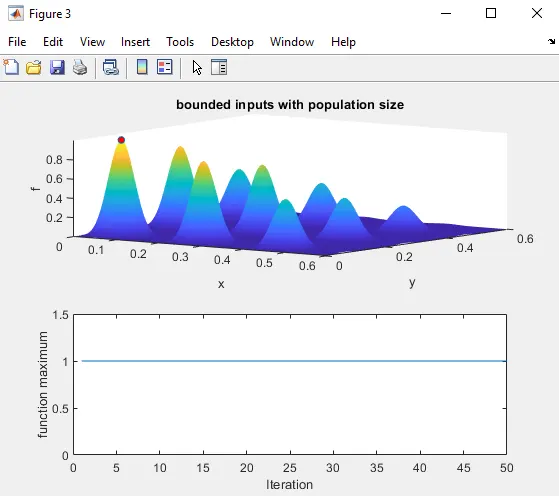
In this iteration the size of the population is increases to global maxima.

clear all
close all
clc
  
%defining our search space
x = linspace(0,0.6,150);
y = linspace(0,0.6,150);

%creating a 2dimensional mesh
[xx, yy] = meshgrid(x,y);

%evaluating the stalagmite function
for i =1:length(xx)
    for j =1:length(yy)
        input_vector(1) = xx(i,j);
        input_vector(2) = yy(i,j);
        f(i,j) = stalagmite(input_vector);
    end
end

%study 3 increasing ga iteration
option = optimoptions('ga','populationsize',200);
tic
num_cases = 50;
for i = 1:num_cases
    [inputs,fopt(i)] = ga(@stalagmite,2,[],[],[],[],[0;0],[0.6;0.6],[],[],...
        option);
    xopt(i) = inputs(1);
    yopt(i) = inputs(2);
end
study3_time = toc
figure(3)
F = -f;
subplot(2,1,1)
hold on
surfc(x,y,F) %generating the surface
shading interp
plot3(xopt,yopt,-fopt,'marker','o','markersize',5,'markerfacecolor','r')
title('bounded inputs with population size')
xlabel('x')
ylabel('y')
zlabel('f')
subplot(2,1,2)
plot(-fopt)
axis([0 50 0 1.5])
xlabel('Iteration')
ylabel('function maximum')
FMAX = -min(fopt);
X = mean(xopt);
Y = mean(yopt);

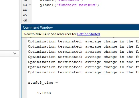
study3_time =

9.1663

error :

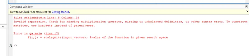
in the stalagmite function.

f1_x = (sin(5.1*pi*x+0.5)).6; power'^' is missing. which is corrected 1_x = (sin(5.1*pi*x+0.5)).^6.

REFERENCES:

https://in.mathworks.com/discovery/genetic-algorithm.html.

https://en.wikipedia.org/wiki/Stalagmite.

https://en.wikipedia.org/wiki/Test_functions_for_optimization.

https://www.tutorialspoint.com/genetic_algorithms/genetic_algorithms_introduction.htm#:~:text=Genetic%20Algorithm%20(GA)%20is%20a,take%20a%20lifetime%20to%20solve..