Assignment 4-RADIOSS Material Laws Challenge
Refer link : https://skill-lync.com/student-projects/radioss-material-laws-challenge-2
ASSIGNMENT 4-
Compare 7 cases as discussed in last 3 slides, in a tabulated format on the basis of:
1. Total number of cycles, Energy error, mass error and simulation time.
2. Notice the animation of all 5 and describe the animations in brief on the
basis of whether the elements are being deleted or cracked.
3. Plot energies and notice any difference.
4. Based on all the results, which case would represent the on-field
scenario.
5. Prepare a ppt/docx and list down case by case result and your conclusion
as to why the failure happened.
Note:
- Refer video titled "Materials 7" for further information
- The 7th case is about LAW 36 and it is explained in the video.
TITLE: RADIOSS Material Laws Challenge
AIM: To run the simulation for a Rigid ball-Plate model using Johnson cook material and elastoplastic material along with brittle failure using Radioss.
OBJECTIVE:
- Run the simulation by changing the material, shell properties and failure parameters.
- Run the simulation by converting Failure Johnson cook material into LAW1.
- Tabulating Energy Error%, Mass Error, SImulation Time & NO. of cycles.
- Simulate for 7 different cases.
INTRODUCTION: In FEA, Generating accurate results is very dependent on having an accurate understanding of the problem being solved, applied loadings, and FEA material properties. Assigning the coorect material along with its material properties is an important factor while performing simulation. The most comprehensive materials along with rupture libraries can be found within Radioss. Material properties can further categorized in two sub cateogeries. They are Material Properties and Material LAWS.
Material LAWS
| LAW 1 | ELASTIC |
| LAW 2 | JOHNSON COOK |
| LAW 27 | ELASTIC-PLASTIC-BRITTLE |
| LAW 36 | ELASTIC-PLASTIC-TABULATED |
| LAW 42 | VISCO-HYPERELASTIC |
| LAW 70 | FOAM |
Material Properties
| ISOTROPIC ELASTICITY |
| ISOTROPIC ELASTO-PLASTIC |
| COMPOSITE & ANISTROPIC |
| VISCOUS |
| HYDRODYNAMIC |
| EXPLOSIVE |
PROCEDURE:
- Firstly, we import the solver deck starter file in hypermesh, once the geometry is loaded we can visualize it.
- switch on shreaded geometry for better resolution.
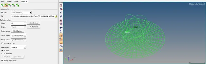
CASE 1: Run the model as it is, rename as law2_epsmax_failure.
- Once the solver deck file is imported, we checkup the geometry, materials, property card.
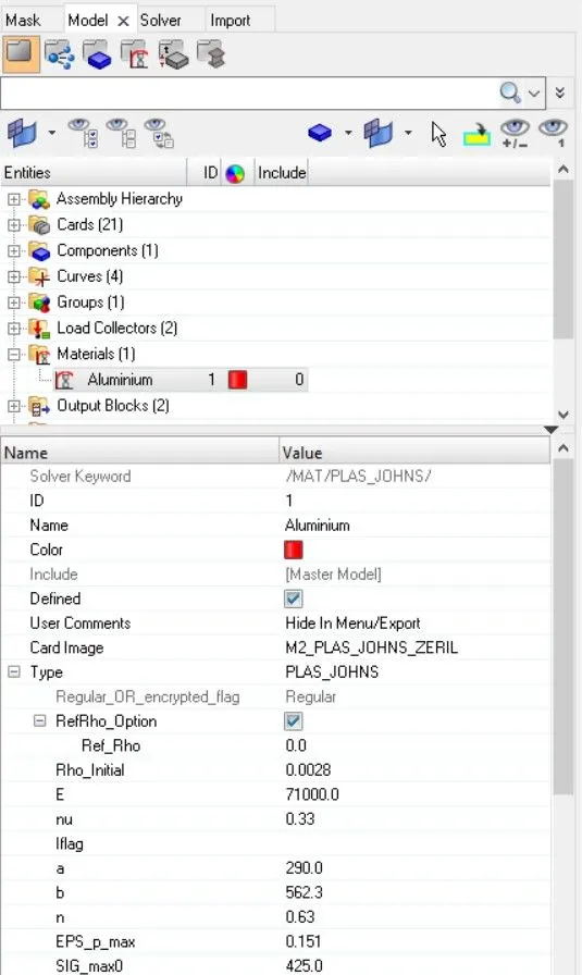
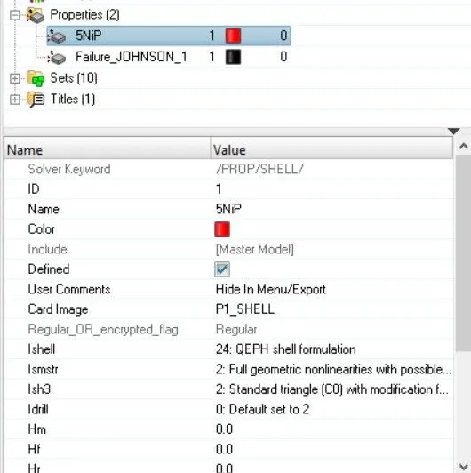
- After they are reviewed, we can proceed with simulation. We hit Radioss in Analysis option.
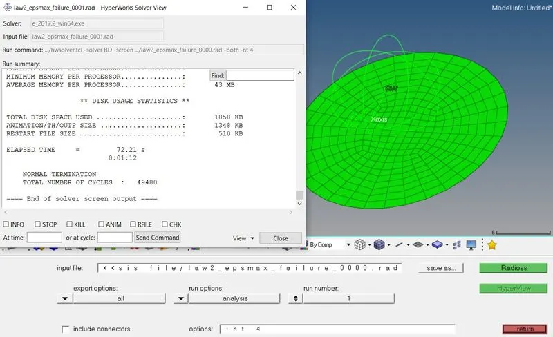
- Simulation window appears and the results are obtained. We check for the Outfile followed by the various graphs, stress,strain values along with parameters such as Energy Error%, Mass Error, SImulation Time & NO. of cycles.
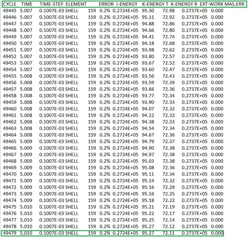
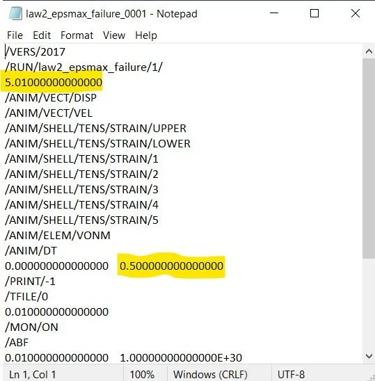
| Energy Error | 0.2% | Internal Energy | 95.27 | Eplased Time | 72.11 | ||
| Mass error | 0 | Kinetic Energy | 0.2724E+05 | Total no. of cycle | 49479 |
- Now, once the results are calculated we load the h3d file in hyperview interface to visualize the animation and the change in the behaviour of elements.
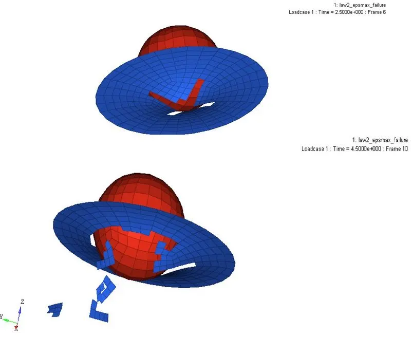
- From above fig, it can be seen that once the rigid ball hits the rupture plate, it went beyond ultimate stress due to which the elements starts to gets delete.
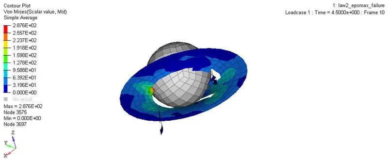
- Then, we plot different graph for the simulation that went through
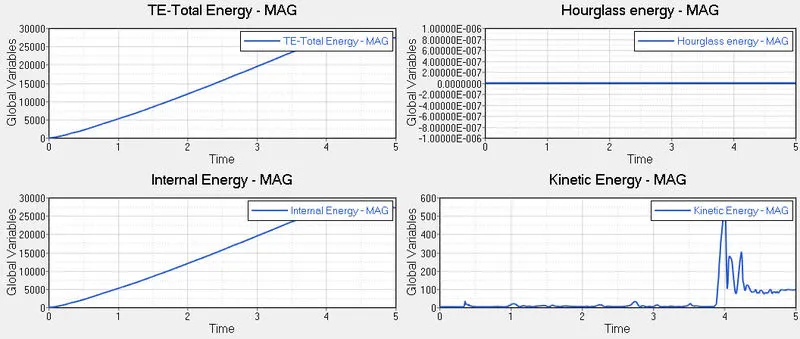
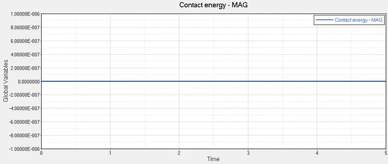
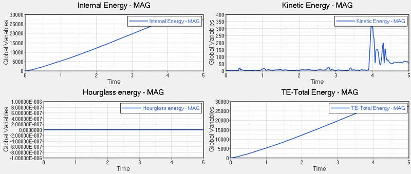
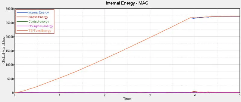
- from above graph, its clear that Total energy is sum of Hourglass energy, kinetic energy , internal energy & contact energy.
- vibration causes the up & down graph in kinetic energy
- since the ridgid wall & plate are elastic they are sort of deformable, so the contact energy plot stays uniform or constant.
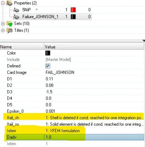
CASE 2: Change the values in Johnson Failure card.
- We ended up changing the material property for the imported solver deck file.
- Here, we assign values as Ifail_shell = 1, DADV = 1, Ixfem = 1.
- Now, we run the solver file as 'LAW2_EPSMAX_FAILURE_0000.rad'
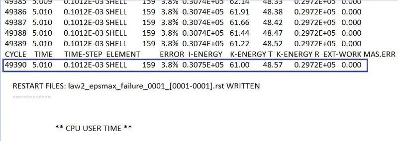
| Energy Error | 3.8% | Internal Energy | 0.3075E+05 | Eplased Time | 48.57 |
| Mass error | 0 | Kinetic Energy | 61.00 | Total no. of cycle | 49390 |
- Once the simulation went through, we have h3d file, which we ended up loading in hyperview interface and the animation can be visualize
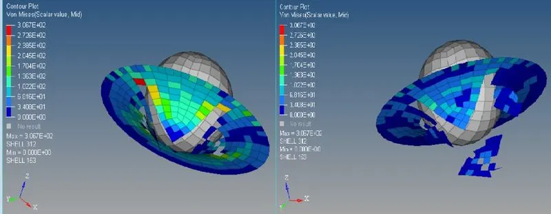
- From above, it is clear that once, the eps_max reaches value of 0.151, the elements start to get delete.
- The elements start to getting repture & deleting further once the rigid wall hits it.
- Finally, we have the graph plots.
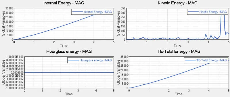
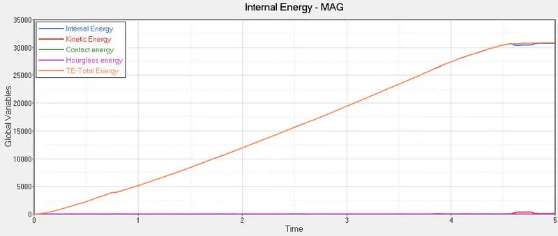
- From Hourglass energy graph, There is no hourglass effect since introduction of Ishell = 24 QEPH it remains constant.
CASE 3: Delete the Johnson Failure Card
- Here, the failure card is deleted in order to see any changes happening in results.
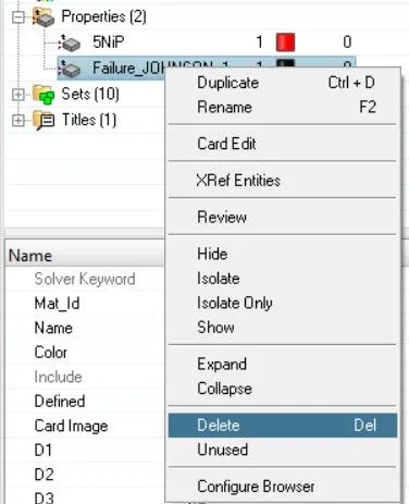
- Then, we simulate using the edited model and proceed for simulation.
- We also take a bit look on the generated values of various parameters.
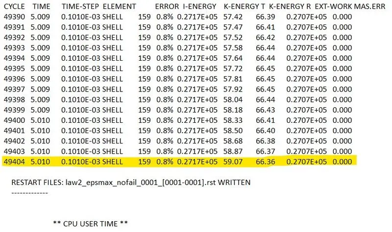
| Energy Error | 0.8% | Internal Energy | 0.2717E+05 | Eplased Time | 66.36 |
| Mass error | 0 | Kinetic Energy | 59.07 | Total no. of cycle | 49404 |
- Once it went through, we go through the h3d file in hyperview.
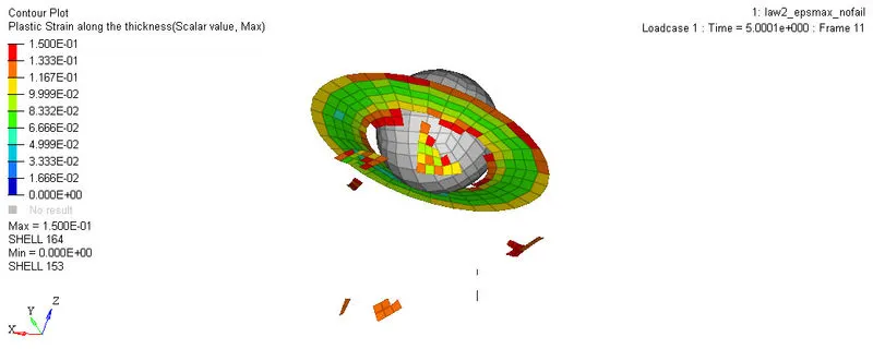
- From above, the shell elements are getteing deleted once they reached maximum plastic strain value.
- Following are the graphs plotted,
CASE 4: Delete the value of EPS_P_MAX & run the mode by name LAW2
- Here, we delete the value for EPS_p_max which is keeping it zero to visualize any changes.
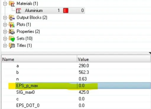
- Then we run the simulation and the desired values are generated.
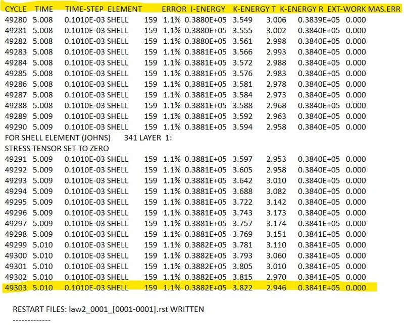
| Energy Error | 1.1% | Internal Energy | 0.3882E+05 | Eplased Time | 2.946 |
| Mass error | 0 | Kinetic Energy | 3.822 | Total no. of cycle | 49303 |
- The simulation can be visualize below,
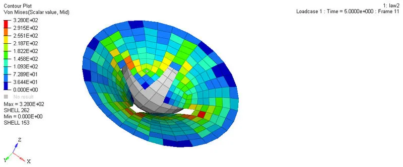
- since the value of EPS_p_max is zero, the elements do not tends to be delete.
- The graph are plotted as follows,
CASE 5: Convert this material model to LAW1 ELASTIC, with same density, E, nu values.
- We assign the LAW1 Elastic material property for the same material followed by keeping the values same.
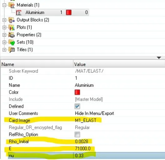
- Once, the simulation is proceed we gets the generated values for desired parameters.
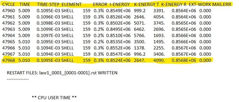
| Energy Error | 0.3% | Internal Energy | 0.8524E+06 | Eplased Time | 4090s |
| Mass error | 0 | Kinetic Energy | 2647 | Total no. of cycle | 47968 |
- The h3d file then is imported in hyperview userface & results are visualize.
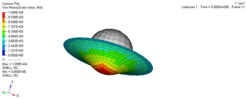
- From above, since the eps value is zero the elements won't be delete.
- The elements won't even splits apart, however LAW1 material is assigned.
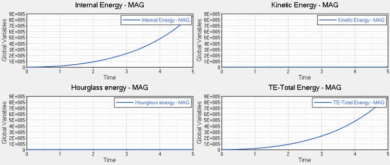
- The T01 file is the imported in hyperview 2d inorder to visualize the graphs
CASE 6: Open LAW27_0000.rad, change the shell property, run using different name.
- As per here, we change the material properties & material law as well.
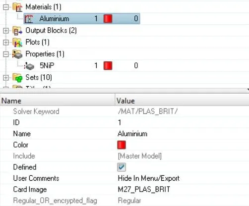
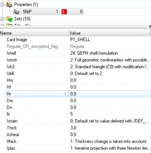
- The moment after the material changes are done, we end up running simulation.
- Once the simulation went through, we acquire the desired values.
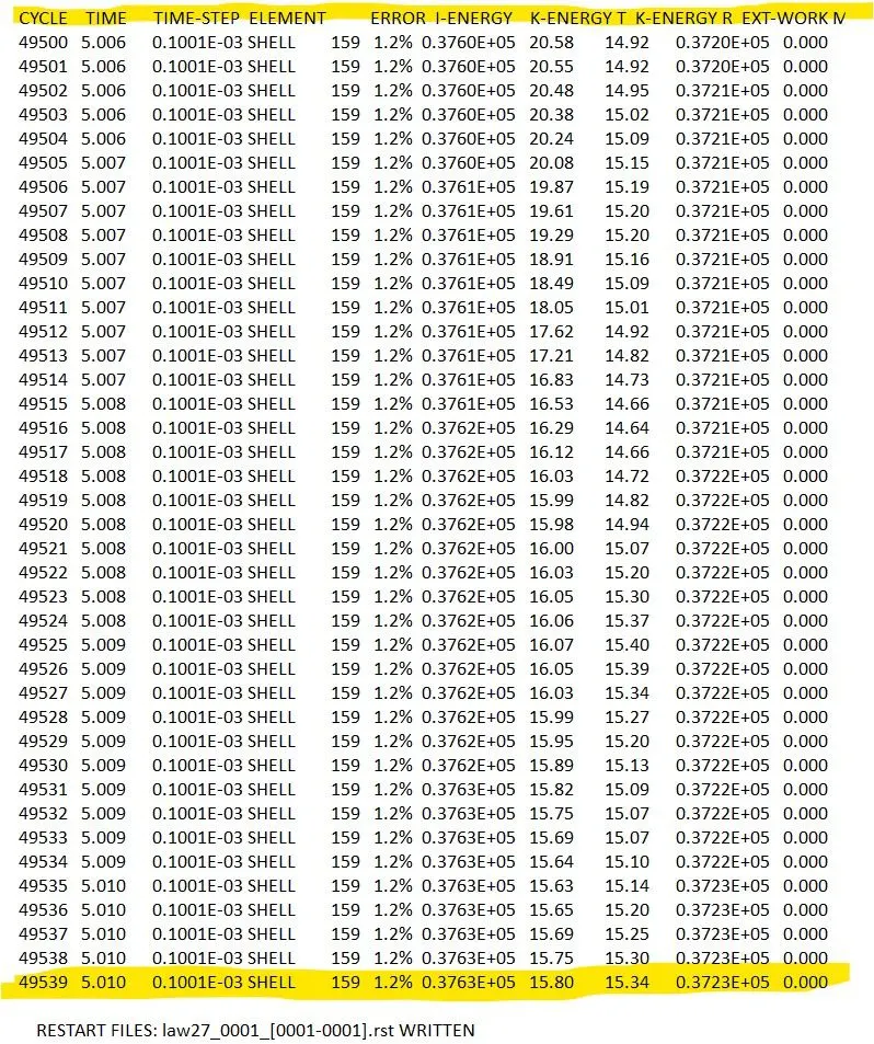
| Energy Error | 102% | Internal Energy | 0.3763E+05 | Eplased Time | 15.34s |
| Mass error | 0 | Kinetic Energy | 15.80 | Total no. of cycle | 49539 |
- The generated h3d file is loaded in hyperview to visualize the simulation.
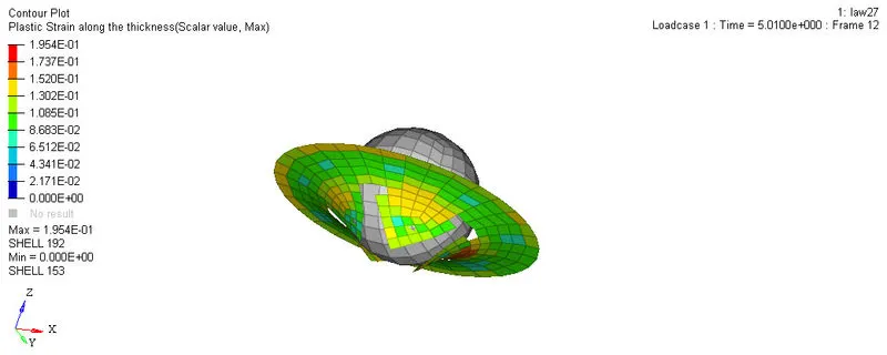
- The LAW27 model is nothing but, isotropic elastoplasto johnson cook model along with orthographic brittle failure model.
- Brittleness resulted in repture of plate as predicted.
- Then, we visualize the graphs.
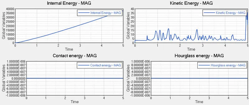
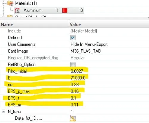
CASE 7: Change the material card to LAW36. along with graph visualizing plastic strain region.
- The solved deck file is loaded, whose material properties has been change to LAW36.
- Its nothing but elasto-plasto piecewise linear material.
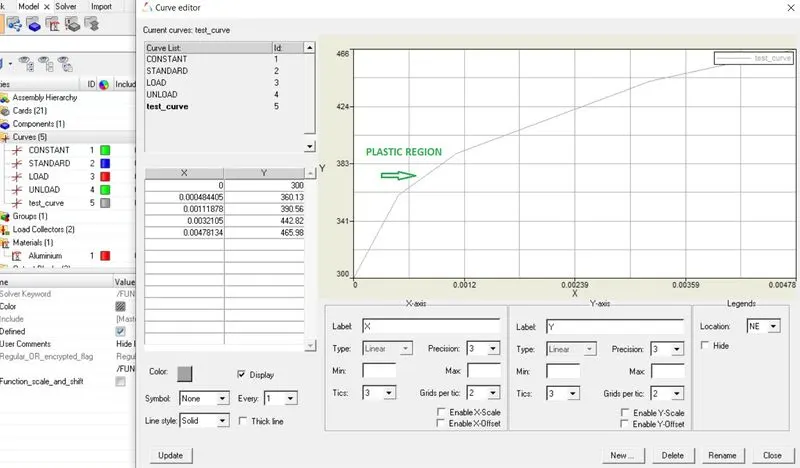
- Then, we also have to define a curve in which the plastic region can be visualize. So we create the curve and values are assigned.
- The curve can be created by assigning the values and the plastic region can be seen as below.
- Then, the simulation is went through and results are acquired.
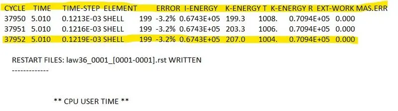
| Energy Error | 3.2% | Internal Energy | 0.6743E+05 | Eplased Time | 1004s |
| Mass error | 0 | Kinetic Energy | 207.0 | Total no. of cycle | 37952 |
- The h3d is the imported in hyperview and the results are visualize.
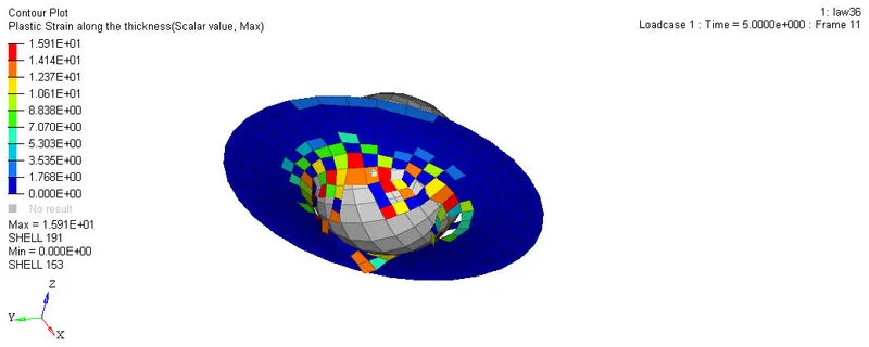
- Here the elements wil be delete once they reach the maximum plastic strain.
- the occurs because they has both elastic as well as plastic property.
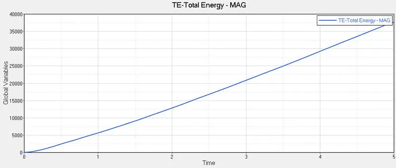
- Then, the Graphs are plotted below.
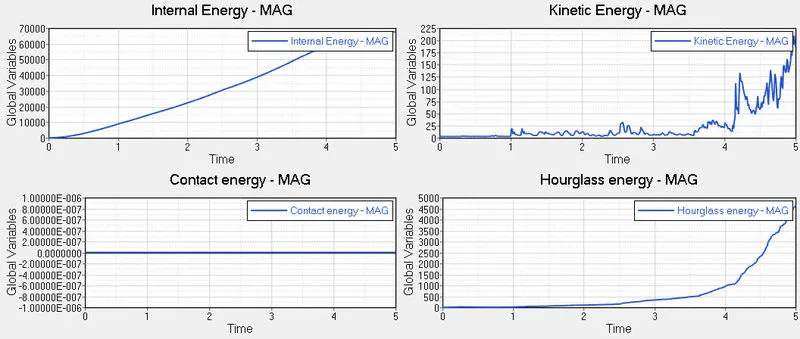
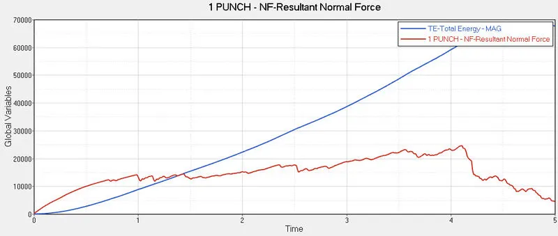
- Comparision of all 7 Cases
| CASE No. | MATERIAL USED | MATERIAL CHANGES | VISLUALIZATION |
| CASE 1 | JHOONSOON COOK LAW2 | DEFAULT RUN | ELEMENTS DELETED |
| CASE 2 | JHOONSOON COOK LAW2 | Ifail_sh,Ixfem, | ELEMENTS CRACKED CRACKED & |
| CASE 3 | JHOONSOON COOK LAW2 | DELETE FAILURE CARD | ELEMENTS DELETED |
| CASE 4 | JHOONSOON COOK LAW2 | Eps_max = 0 | ELEMENTS DEFORMED |
| CASE 5 | ELASTIC LAW 1 | CHANGE TO LAW1 | ELEMENTS DEFORMED |
| CASE 6 | ELASTO-PLASTO BRITTLE | INTRODUCE BRIITLE | ELEMENTS DELETED |
| CASE 7 | ELATO-PLASTO-TABULATED | INTRODUCE PLASTIC STRAIN CURVE | ELEMENTS DELETED |
RESULTS & CONCLUSION:
- The simulation consisting all 7 different cases went through.
- THE LAW36 is more suitable, however it provides both elastic as well as plasticity.
- studied elements behaviour on repture & delete.
- Defined a plastic strain region on a graph
- By changing the material properties, law the desired results are being change more frequently.
- Studies failure criteria