Assignment 4-RADIOSS Material Laws Challenge

Aim

Comparison of results with LAW 2 , failure mode and LAW 27 with different materials cases

Objective

To carry out simulation of the given starter file and compare the results. there shall be 7 cases (according to given parameters) and they are to be compared primarily via animation and plots. the files to be worked on are the FAILURE_JOHNSON_0000.rad file and Law27_0000.rad file. the cases are as follows:

1. LAW 2 file(FAILURE_JOHNSON_0000.rad) base simulation
2. LAW 2 file(FAILURE_JOHNSON_0000.rad) with Ifail_sh = 1, Dadv = 1 and Ixfem = 1
3. LAW 2 (file: starter file for case 2) with fail/JOHNSON card deleted
4. LAW 2 (file: starter file for case 3) with EPS_p_max value deleted
5. LAW 1 (file: FAILURE_JOHNSON_0000.rad) with fail/JOHNSON card deleted and value for density,E,Nu assigned
6. LAW 27 (file LAW27_0000.rad) with recommended shell properties with different value for EPS based failure
7. LAW 36 (file LAW27_0000.rad) with recommended shell properties and given reference curve.

Indroduction

•  The accuracy of the simulation depends on the materials and analysis type choosen 
• Radioss has multiple material properties and wide variety of material library like concrete. foam,rubber, composites and so on
• Commerically used material laws are:-

1. Law 1: Elastic(Isotropic Elasticity)
2. Law 2: Johnson-cook(Isotropic Elasto-plastic)
3. Law 36: Elastic-plastic Tabulated
4. Law 27: Elastic-plastic brittle
5. Law 42: Ogden(viscous hyperelastic)
6. Law 70: Foam

Law 1: Elastic(Isotropic Elasticity)

The Elasticity law follow the hook's law of elasticity i.e a linear relationship between stress and strain. the material stiffness is determined by Young's modulus of elasticity (E) and poisson's ratio.

Limitation 

• Elastic materials cannot be used for large deformation cases such as blow molding
• In the case of large deformation, Law 2 Johnson-cook material with high yield can be used 

Law 2: Johnson-cook(Isotropic Elasto-plastic)

Radioss provides various types of elasto-plastic material laws. It has all the materials models based on von mises hardening without damage, von mises hardening with ductile damage, von mises with visco-plastic flow

• This law represent an isotropic elasto-plastic material using the johnson-cook material model
• The model express material stress as a function of strain, strain rate and temperature
• In the material card we have EPS_max which is plastic strain at failure. failure of the element happens when 1 integration point reaches EPS_max.Now if failure is only based on EPS_max, there can be instances where the EPS_max gives unrealistic result. to avoid this, we have option called /FAIL/JOHN, This FAIL/JOHN card provides the user with more control over the failure of the Johnson-cook strain.

Law 36: Elastic-plastic Tabulated (Elastic plastic piecewise linear material)

• The law 36 materials helps in modeling isotropic elasto-plastic material using user defined functions for the work hardening portion of the stress- strain curve for different strain rates.
• The curve defined is nothing but the stress- strain curve after the yield point. The yield point is set to 0
• This material law is availabe for both brick and shell elements
• If the work hardening portion is defined by the user, then its elastic portion is taken from the inputted young's modulus and poisson's ratio.
• Law36 model has 4 damage and repture parameters

Law 27: Elastic-plastic brittle

• This Law27 has isotropic elasto-plastic material law with orthotropic brittle failure model. Orthotropic materials differ along three mutually-orthogonal axes
• Here, the material damage and failure happens only in tension
• Same as Law36, this material law also have damage and failure parameters 

Procedure

CASE 1: LAW 2 file(FAILURE_JOHNSON_0000.rad) base simulation 

Import CAD geometry

The first step is to open the HyperWork software and in the interface it will ask to select the a solver, here we select Radioss as a solver. Then we need to import the FAILURE_JOHNSON_0000.rad file.

Than go to file ->import->select the component from directory and click import 

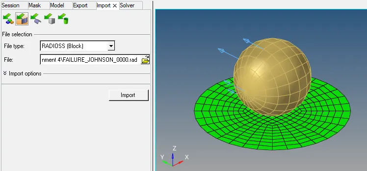
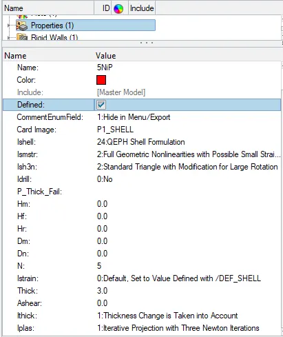
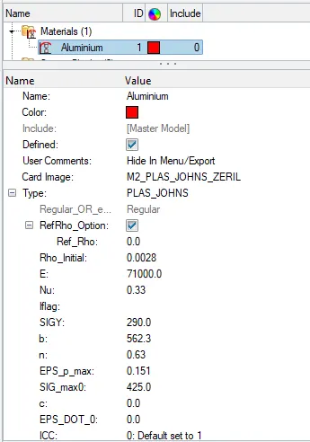
See the material and properties of default value

  

To run the simulation, Go to Analysis->Radioss. Save the file as "Law2_espmax_failure.0000.rad". In option type -nt 4 which means assigning the task to 4 cores in the system, to perform the simulation faster.its depends upon the process of iur computer(it has a quad- core processor, than it will take as 4. if the system has an octa- core processor than it is taken as 8). nt means number of threads, finally click on Radioss in order to run the simulation.

After clicking Radioss we get the solver window as shown below, after few minutes Radioss does the job and click on Result 

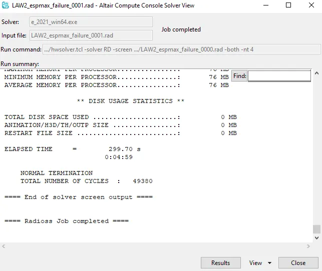
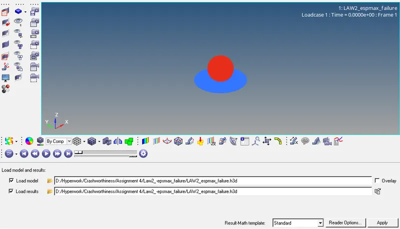
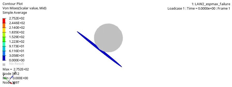
 After Clicking on result it will switch to Hyperview window.Now on Hyperview we should input the the simulation file for this we use .h3d file that was generated when Radioss Processed the starter file(LAW2_espmax_failure.h3d) after selecting it click on apply. Now to simulate the animation click on contour option in the toolbar. change the result types to von mises stress and change average method to simple click on apply. Animation will start as shown below

Now its time to energy error and mass error check and this is done by analyzing the radioss engine output file. it can be accessed from the same directory as the starter and engine file and it ifile extension by _0001.out open this file in notepad as shown below.

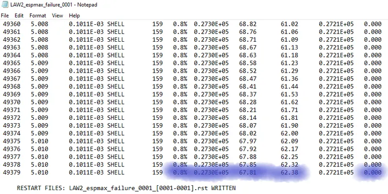
The final energy error is 0.8% which is in the range of -15% to +5%,which is closer to zero, which is very acceptable. there is no mass error. 

Post processing

• Switch to Hypergraph 2D to plot the different energy 
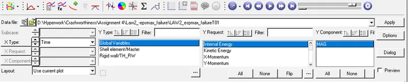
• In Hypergraph 2D section we need to input a file called_T01 file as shown below

• In this first case, it has FAIL/HOHNSON card as well as ESP_P_max value assign with Ixfem = 0. This mean elements will deleted as soon as they cross EPS_max threshold which we can see below simulation.

             

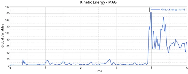
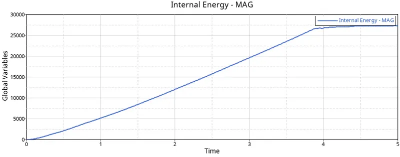
• Internal energy as well as rigid wall forces are reaction to the force generated by the sphere on the sheet . Energy increases linearly untile a large mnumber of elements are deleted at round the 4 ms threshold. This probably creates some vibration and that results in a surge of kinetic energy at the same point.

      

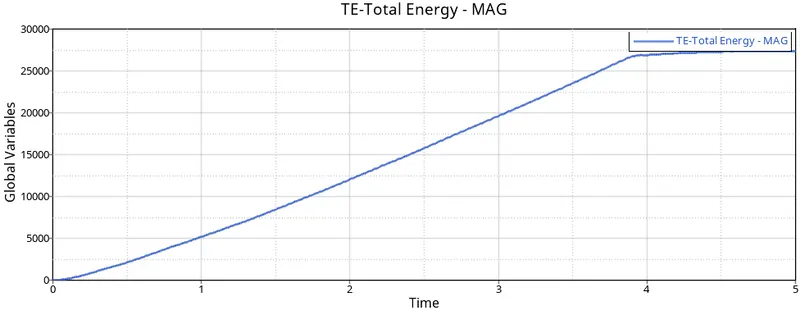
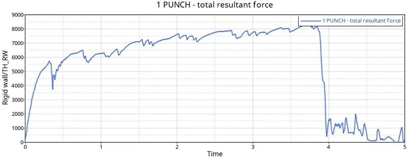
The rigid wall forces fluctuate due to element deletion and when a large chunk of elements are deleted at 4 ms, the graph drops, meaning there aren't many elements opposing the force of the sphere. Most of the elements in its path been deleted at that point.

CASE 2 LAW 2 file(FAILURE_JOHNSON_0000.rad) with Ifail_sh = 1, Dadv = 1 and Ixfem = 1

• The process is repeated with slightly changes. Similar to case1, we import FAILURE_JOHNSON_0000.rad via solver deck import process.
• This time we make some changes to fail/JOHNSON card.it canbe access via the modeltab, under failure submenu.click on Failure_JOHNSON_1 and  substitude the value of Ifail_sh = 1, Dadv = 1 and Ixfem = 1 as shown below.

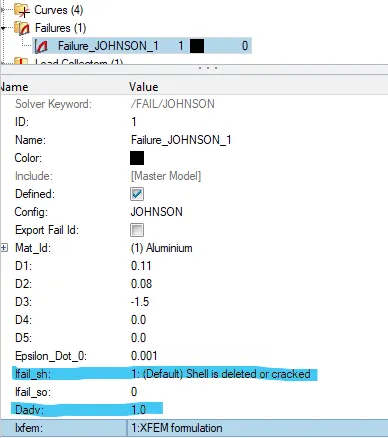
Ifail = 1 which determines the shell element failure method. so there are two way in which we can see the element  failing, the elememt will either get deleted or in some cases the cracking will occurs according to material properties.

Dadv = 1

It get activated when we have taken Ixfem = 1. we are going to take Dadv = 1. which gives the criteria that how an element can get break into small pieces. if it goes beyond  the limit the element gets delete.

Ixfem = 1 

In this,we can choose that if there is any element that is failing we want that element to delete or we want the element to be crack. we are going to take Ixfem = 1, which allow failed element to cracked not to delete.

• After the value are assigned, we continue as in previous case by letting the Radioss engine run the analysis.This is done via Analysis-> Radioss. This time the file is saved as LAW2_espmax_crack_0000.rad. click on Radioss. After the solver window completes the analysis click on result 
• After Clicking on result it will switch to Hyperview window. Now on Hyperview we should input the the simulation file for this we use .h3d file that was generated when Radioss Processed the starter file(LAW2_espmax_crack.h3d) after selecting it click on apply. Now to simulate the animation click on contour option in the toolbar. change the result types to von mises stress and change average method to simple click on apply. Animation will start as shown below

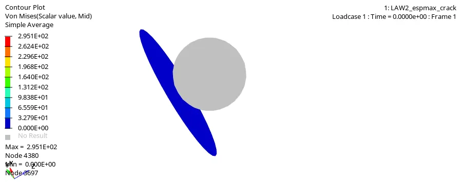
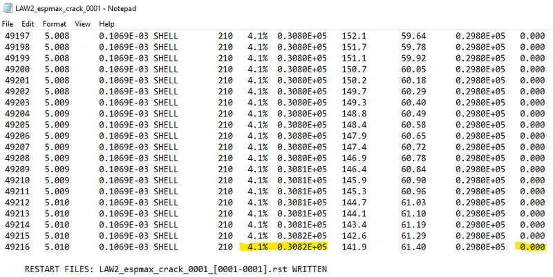
The final energy error is 4.1% which is in the range of -15% to +5%,which is closer to zero, which is very acceptable. there is no mass error. 

Post processing

Case 2 makes use of Ifail_sh, Dadv and Ixfem as part of the fail/JOHNSON card. Ixfem is especially important here because it decides the way the element react. with its value equal to 1, it means the elements will crack and fail. Along with Dadv, crack propagation can also reaches them. As a result, this is a more realistic depiction.

   

   

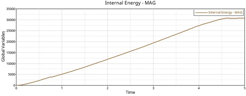
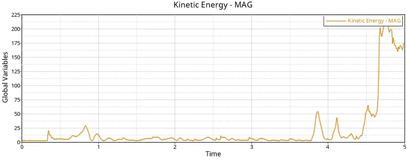
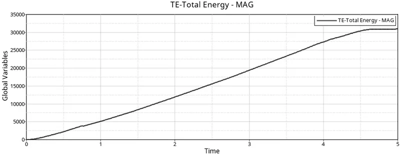
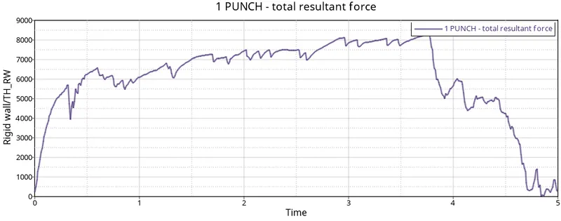
It can be noticed that in both case 1 and 2, the internal energy graphs are almost same. They differ when it comes to the timestep at which they pleatea and this is probably due to crack propagation being a big factor in case 2. The instant deletion in case 1 as compare to energy dissipation dure to crack in case 2 creates the different.

CASE 3 LAW 2 (file: starter file for case 2) with fail/JOHNSON card deleted

• Again, we need to switch to hyperwork and import the solver deck file for this case, LAW2_espmax_crack_0000.rad is imported as the starte file created in previous case.
• In this case delete the fail/JOHNSON card. Go to model->failure->Failure_JOHNSON as shown below

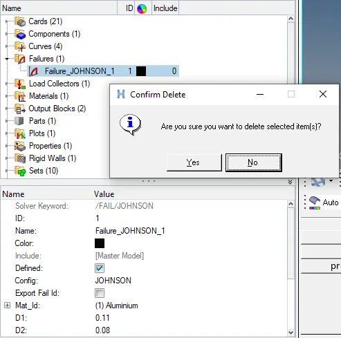
• Now run the analysis and save the file as "Law2_espmax_nofail_0000.rad". click on Radioss. After the solver window completes the analysis click on result 
• After Clicking on result it will switch to Hyperview window. Now on Hyperview we should input the the simulation file for this we use .h3d file that was generated when Radioss Processed the starter file(LAW2_espmax_nofail.h3d) after selecting it click on apply. Now to simulate the animation click on contour option in the toolbar. change the result types to von mises stress and change average method to simple click on apply. Animation will start as shown below

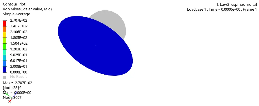
 Now check the energy and mass error on Radioss output file Law2_espmax_nofail_0001.out. open this in notepad 

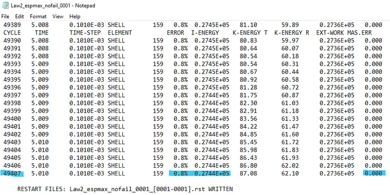
 The energy error is 0.8% amd mass error is non existent. Now we can switch to Hypergraph 2D to plot the graphs.

Post processing

• With the fail/JOHNSON card deleted in this case. the EPS_p_max to be factor for element deletion. its value is 0.151 meaning elements will be deleted if the strain on any integration point within said elements reaches 15.1 % of the plastic strain.The element in this case, fail rapidly when compared to case 2 due to Ixfem crack formulation there. 

   

   

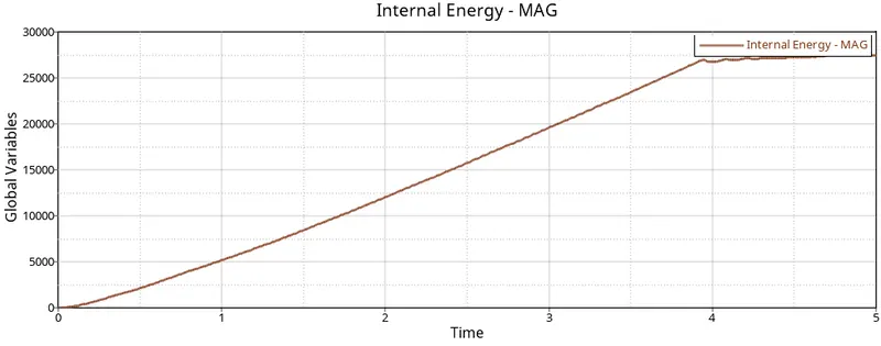
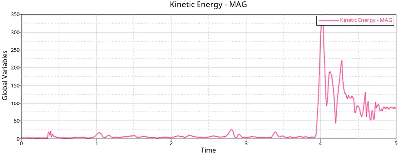
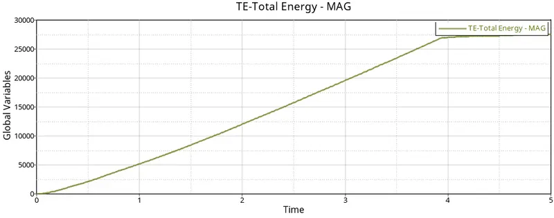
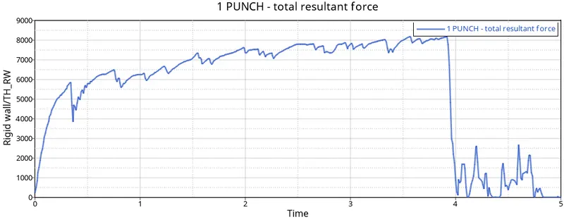
• There is linear increase in internal and total energy until a bulk of the elements are deleted from the model. This is expected since the energy absorbed by these elements go to waste due to their deletion.
• This also explain the sudden drop in rigid wall forces at the same timestep due to most elements that were in contact with the sphere during collision being deleted. fluctuations occur when elements are deleted.

CASE4: LAW 2 (file: starter file for case 3) with EPS_p_max value deleted

•  In this case, import the case 3 starter file Law2_espmax_nofail_0000.rad. 
• This time delete the EPS_p_max value( EPS_p_max = 0).Go to model tab ->materials->Aluminium as shown below

  

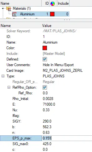
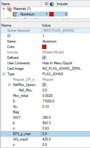
• Now run the analysis and save the file as "Law_2_0000.rad". click on Radioss. After the solver window completes the analysis click on result 
• After Clicking on result it will switch to Hyperview window. Now on Hyperview we should input the the simulation file for this we use .h3d file that was generated when Radioss Processed the starter file(LAW_2.h3d) after selecting it click on apply. Now to simulate the animation click on contour option in the toolbar. change the result types to von mises stress and change average method to simple click on apply. Animation will start as shown below

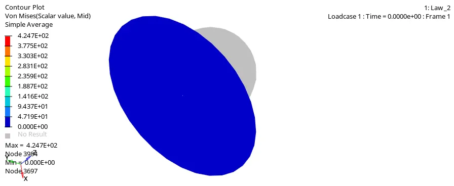
Now, check the energy and mass error on Law_2_0001.out

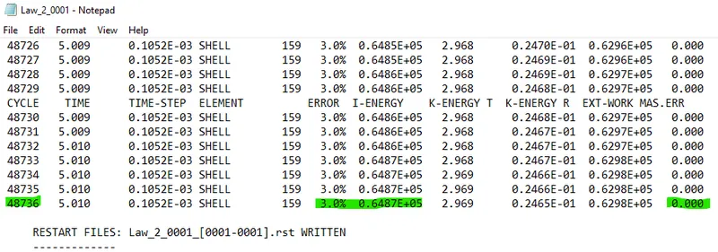
The energy error is less than 5% and mass error non-existent.

Post processing

The metal sheet ia able to withstand a large amount of stress and avoid element deletion primarily dure to the fact that the value of EPS_p_max was deleted.since it is deleted, Radioss assigns it default value of 10^30. in addition to that, the fail/JOHNSON card was deleted.the material behaves like a pseudo-elastic(also called elesto-plastic) material since it has a very high EPS_pmax threshold and elements cannot be deleted to failure cards.

With the value of c(strain rate coefficient)=0, there is no strain rate(neither does temporary play a role here). As the result, the stress in this case is purely a function of strain generated in the materials.

 

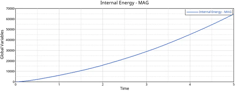
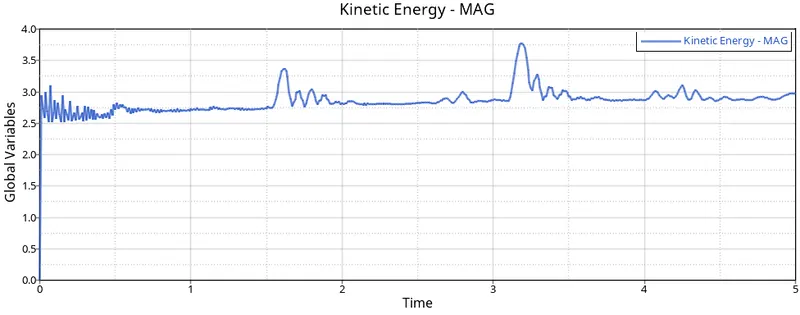
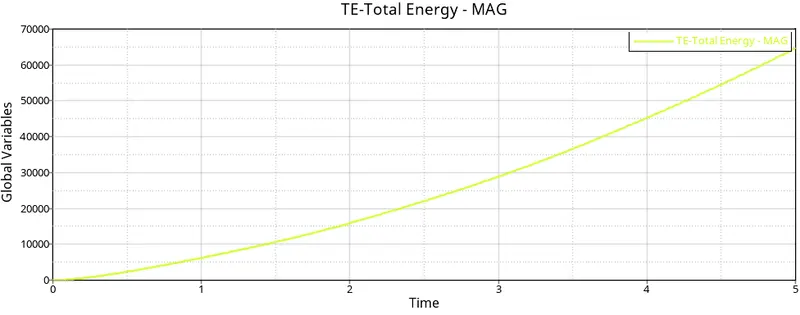
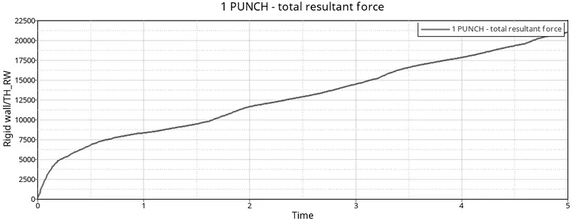
Added, the kinetic energy generated in this case is almost negligible(2.5-3.75mJ) compare to internal and total energy.The total energy is almost linear over time.

CASE 5: LAW 1 (file: FAILURE_JOHNSON_0000.rad) with fail/JOHNSON card deleted and value for density,E,Nu assigned

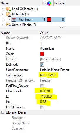
• In this case import main starter file-FAILURE_JOHNSON_0000.rad. After that go to material card change the material card to M1_ELAST (Law1) and set the value of Rho_initial, E and Nu as follow: 0.0028, 71000 and 0.33 respectively.

• Now run the analysis and save the file as "Law_1_0000.rad". click on Radioss. After the solver window completes the analysis click on result 
• After Clicking on result it will switch to Hyperview window. Now on Hyperview we should input the the simulation file for this we use .h3d file that was generated when Radioss Processed the starter file(Law_1.h3d) after selecting it click on apply. Now to simulate the animation click on contour option in the toolbar. change the result types to von mises stress and change average method to simple click on apply. Animation will start as shown below

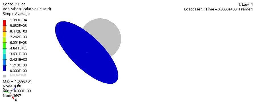
 Now, check the energy and mass error on the Radioss output file Law_1_0001.out

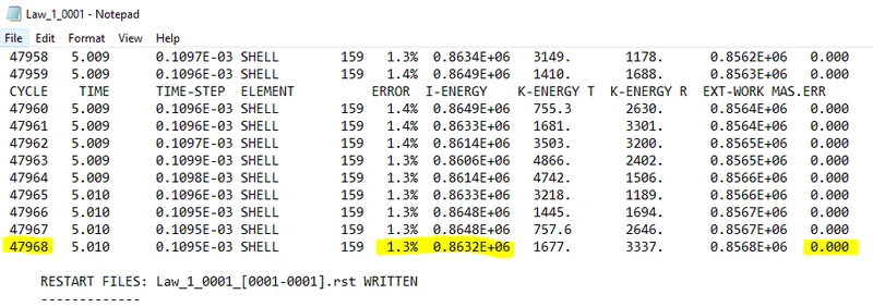
 The energy error is less than 5% and masss error is non existent. we can switch to Hypergraph to plot the graphs.

 Post processing

In this case, the plate ids defined with a LAW1 material which defines the basicc properties of elastic materials. This model considers only the elastic phase of th material, there is no plasticity involved which result in linear deformation.

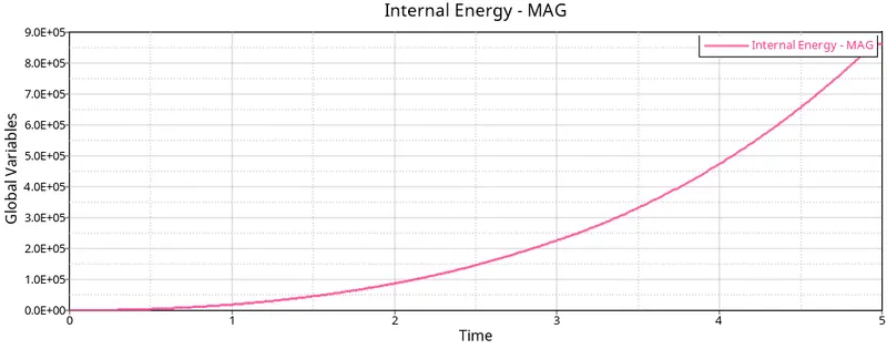
This case make use of M1_Elast card and as we can see, the metalsheet absorbs the full impact of the sphere. this material law is used to model purely elastic materials. this explains why there is no element deletion or ruptures.

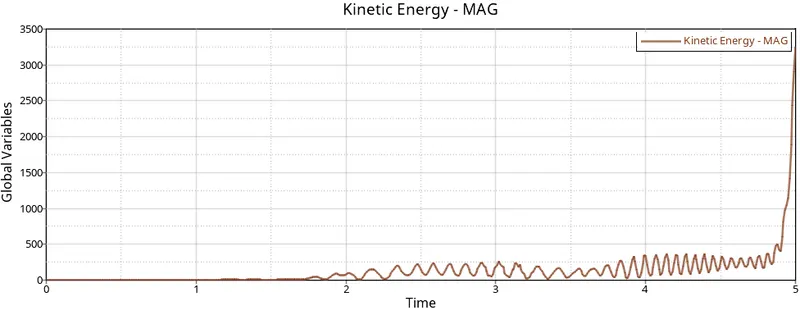
Kinetic energy gradually increases as the plate is stretched to the maximum limit for the applied load.

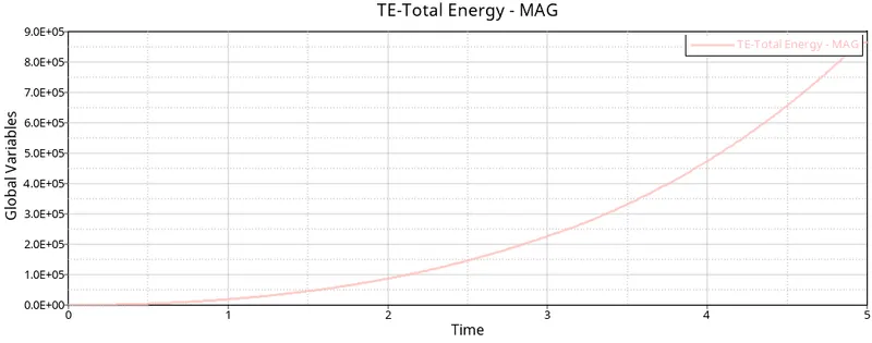
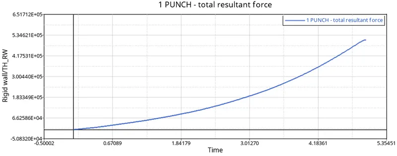
Due to the elastic nature, the internal energy and rigid wall force keep increases exponentially. The internal energy of the metal sheet increases due to the absorption of the kinetic energy from the impacting sphere and drops down once the plate return to the original shape.

CASE6: LAW 27 (file LAW27_0000.rad) with recommended shell properties with different value for EPS based failure

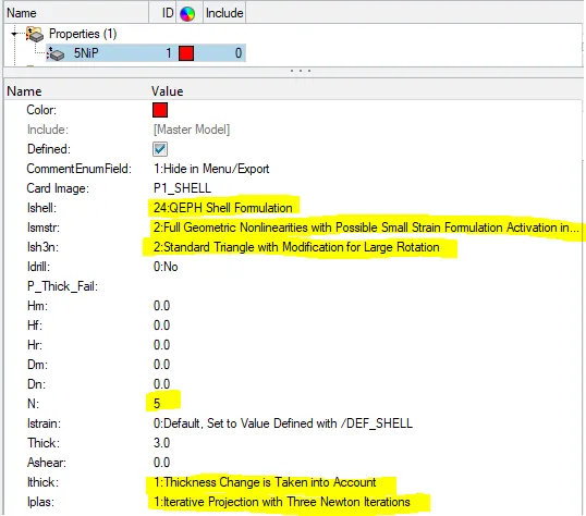
In this case, import the Law27_0000.rad file. we need to used recommended shell properties in this case. Go to properties->5NiP and change shell properties as shown below

• Now run the analysis and save the file as "Law_27_0000.rad". click on Radioss. After the solver window completes the analysis click on result 
• After Clicking on result it will switch to Hyperview window. Now on Hyperview we should input the the simulation file for this we use .h3d file that was generated when Radioss Processed the starter file(Law_27.h3d) after selecting it click on apply. Now to simulate the animation click on contour option in the toolbar. change the result types to von mises stress and change average method to simple click on apply. Animation will start as shown below

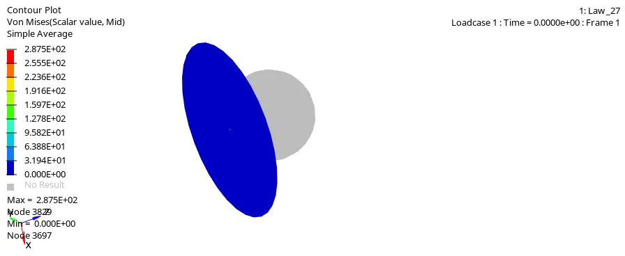
Now, check the energy and mass error on the Radioss output file Law_27_0001.out

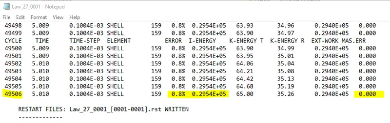
Now, we can see the energy error less than 5% and mass error is non existent. we can switch to Hypergraph to plot the graphs.

Post processing

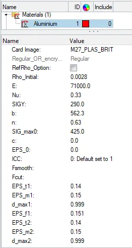
In this case the uses of M27_PLAS_BRIT material card that is used for isotropic elastoplastic Johnson-cook material model with an orthotropic brittle failure model. the sheet (compare to case 7) absorbs more force and resort to more deformation before the elements are deleted (at around 4 ms)

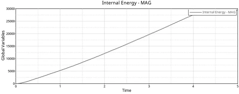
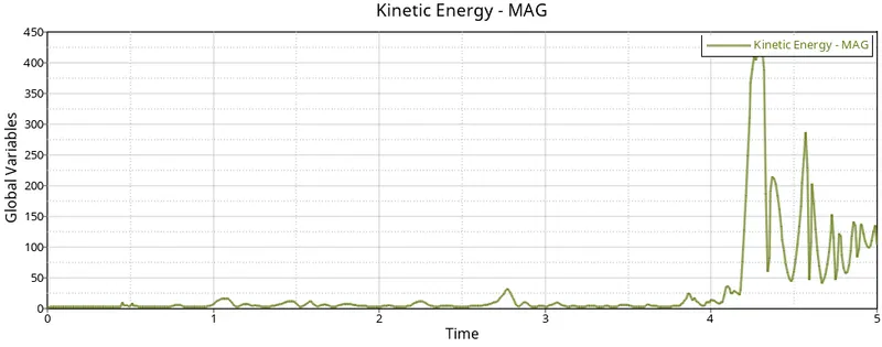
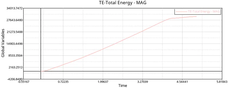
With several elements deleted and non to stop the incoming sphere, the rigid wall force graph drops at the same timestamp of 4ms. The spike are formed when an element is deleted and is characterized by a trough and crest but with so many elements deleted, the trough is massive at 4ms. 

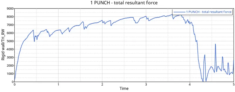
case7: LAW 36 (file LAW27_0000.rad) with recommended shell properties and given reference curve.

 In this case import Law27_0000.rad starter file again. we shall be editing attributes in this case 

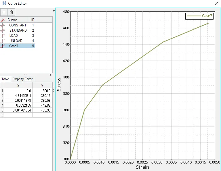
Go to model tab-> right click on curves->create-> curve as per given data.

initially there are 4 curves, we are adding the new curve named as case7 and enter the value as shown below

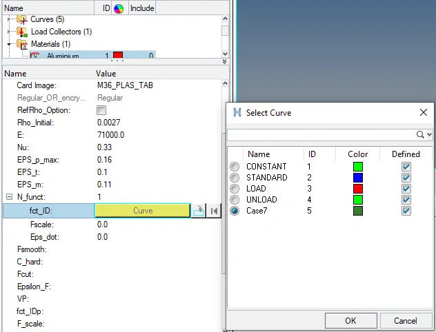
 Go to materials-> Aluminium and change the card to M36_PLAS_TAB(Law 36) afer that set the value of Rho_initial,E,Nu as 0.0027,71000,0.33 respectively.

 

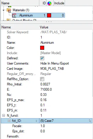
Now run the analysis and save the file as "Law36_0000.rad". click on Radioss. After the solver window completes the analysis click on result 

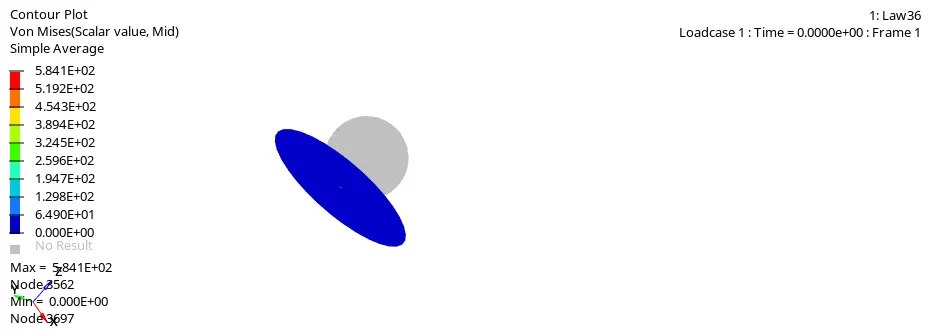
After Clicking on result it will switch to Hyperview window. Now on Hyperview we should input the the simulation file for this we use .h3d file that was generated when Radioss Processed the starter file(Law36.h3d) after selecting it click on apply. Now to simulate the animation click on contour option in the toolbar. change the result types to von mises stress and change average method to simple click on apply. Animation will start as shown below

Now, check the energy and mass error on the Radioss output file Law36_0001.out

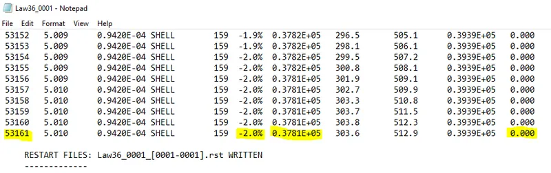
An energy error of -2% is very acceptable since it's very close to zero. as usual, mass error os non-existent. Now we can switch to Hypergraph to plot the graph

Post processing

In this case, from the simulation, we can say that this material exhibits strong brittle behaviour. it does not bend as much in response to the applied force and immediately disintegrates. There seems to be not much cracking and the region of element deletion takes the shape of the sphere. Another thing thate we can notice is that the stress concentraction is localized around the region of impact and these stress are not dissipated throughout the whole metal plate.

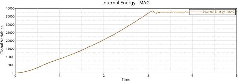
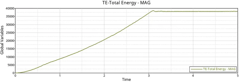
There is an almost linear relation between internal energy and time till past the 3 ms where many elements get deleted at onc, Where the element are deleted, the energy on each element goes to waste.

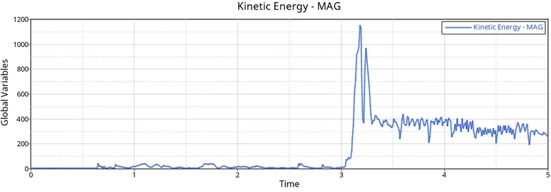
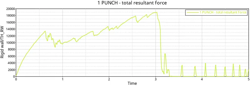
On the topic of energy wastage and element deletion, it is more particular visible in the rigid wall force graph. Each of the spikes is due to an element deletion.The resultant force gradually increases past the same 3 ms which is when the sheet gives way and lets the sphere through. with not much of the sheet in the way, the rigid force are drastically reduced. 

Comparision 

Hourglass Energy in all the cases remain almost zero.

CASE	Solver simulation processing time in second	Number of cycle	Mass Error	Final Energy Error	Von mises stresses	Condition of elements under excessive stress
LAW 2 file(FAILURE_JOHNSON_0000.rad) base simulation	299.70	49379	0	0.8%	275.2 MPa	Elements are deleted without crack formation
LAW 2 file(FAILURE_JOHNSON_0000.rad) with Ifail_sh = 1, Dadv = 1 and Ixfem = 1	368.98	49216	0	4.1%	295.1 MPa	Elements undergoes crack formulation and then deletion
LAW 2 (file: starter file for case 2) with fail/JOHNSON card deleted	421.39	49407	0	0.8%	270.7 MPa	Deleted
LAW 2 (file: starter file for case 3) with EPS_p_max value deleted	312.30	48736	0	3%	427.7 MPa	Cannot be deleted due to lack of failure card and default EPS_p_max value
LAW 1 (file: FAILURE_JOHNSON_0000.rad) with fail/JOHNSON card deleted and value for density,E,Nu assigned	386.13	47968	0	1.3%	10890 Mpa	Cannot be deleted  due to elastic card property
LAW 27 (file LAW27_0000.rad) with recommended shell properties with different value for EPS based failure	311.06	49506	0	0.8%	287.5 MPa	Deleted
LAW 36 (file LAW27_0000.rad) with recommended shell properties and given reference curve.	316.85	53161	0	-2.0%	584.1 MPa	Deleted

Learning outcomes

• Able to understand assign material parameter
• Learn about internal, kinetic, contact and total energy also hourglass energy
• Able to perform different cases simulation 
• Learn about failure card

Conclusion

Selecting a correct material model play a very vital role in simulation and analysis

Law1 is used to model purely elastic materials that remain in the elastic range, follow Hook's Law

Law2: In this law, the material behaves as linear elastic when equivalent stress  is lower than the yield stress. for higher value of stress , material behave like plastic. failure can be capture better with the help of an optional fail_Johnson card

Law27 used for brittle materials

Law36: The elastic-plastic behaviour of isotropic material is model with user defined function. This stress and strain curve is modeled using E and Nu. Therefore,this is best card because we cannot know the exact failing condition of the material in the other cases, but we can define the stress-strain curve and then we can decide where the material is failing.