Assignment 4-RADIOSS Material Laws Challenge

Objective:

Comparison of results with various cases of material laws.

1.Law2_epsmax_failure

2.Law2_epsmax_crack

3.Law2_epsmax_nofail

4.Law2

5.Law1

6.Law27

7.Law36

Procedure:

1. Law2_epsmax_failure

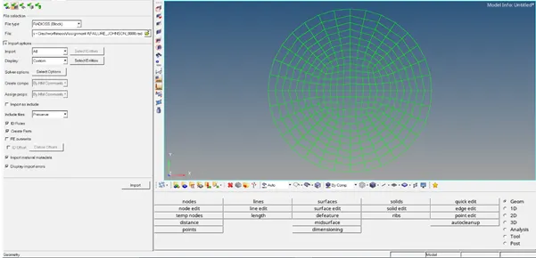
Import FAILURE_JOHNSON_0000.rad file in hypermesh(Solver Deck).

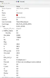
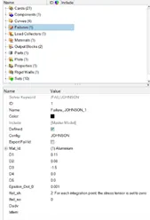
Check the properties and failure cards of the imported file.

In Analysis panel, select Radioss and save the input file as Law2_epsmax_failure_0000.rad in a separate folder (to save the animation files), mentioning the option = “-nt 4”.

Then run the input file, by selecting Radioss to perform the simulation.

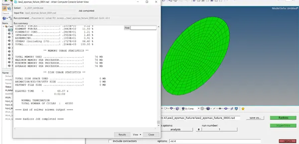
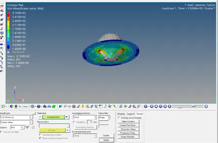
Select Results, to view the simulation – Select the Contour for displacement, von mises and save the files.

Go to Hypergraph, 2D to plot the desired graph for comparison.

Total Resultant Force:

Internal Energy:

Kinetic Energy:

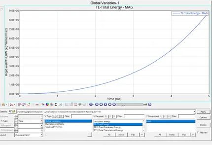
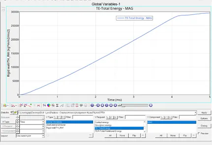
Total Energy:

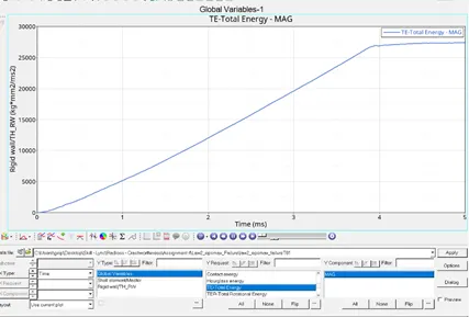
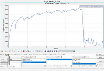
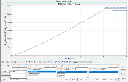
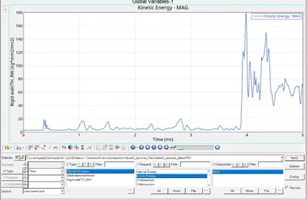
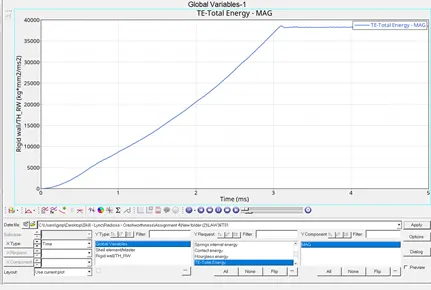
The model has both Failure and eps_p_max(Ixfem=0), during simulation elements are gets cracked and thrown away after 4ms (threshold), up to this threshold internal energy is increasing linearly and then stays constant, whereas kinetic energy shows some large vibration during the threshold also we can see that the rigid wall force also fluctuates at this threshold, due to the elements are getting cracked & deleted.

2.Law2_epsmax_crack

Import FAILURE_JOHNSON_0000.rad file in hypermesh(Solver Deck).

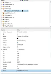
In failure card, Failure_JOHNSON_1 change the values (Ifail_sh=1, Dadv=1, Ixfem=1).

In Analysis panel, select Radioss and save the input file as Law2_epsmax_crack_0000.rad in a separate folder (to save the animation files), mentioning the option = “-nt 4”.

Then run the input file, by selecting Radioss to perform the simulation.

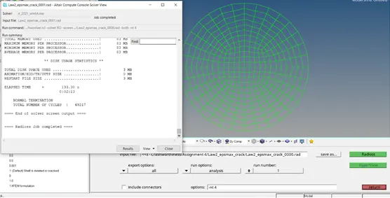
Select Results, to view the simulation – Select the Contour for displacement, von mises and save the files.

Go to Hypergraph, 2D to plot the desired graph for comparison.

Total Resultant Force:

Internal Energy:

Kinetic Energy:

Total Energy:

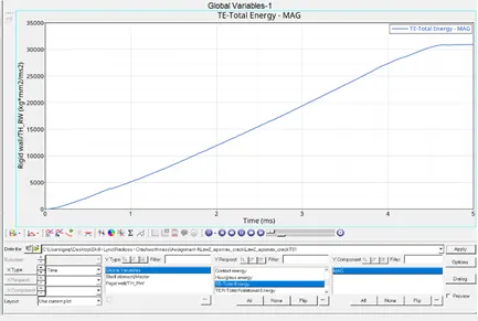
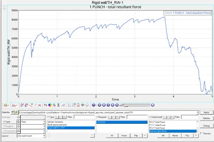
Model have Ifail_sh, Dadv, Ixfem defined in Failure_JOHNSON_1, From the simulation, it is observed that the elements are deleted only after the propagation of crack reaches them.

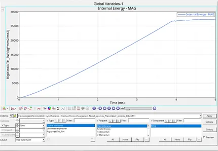
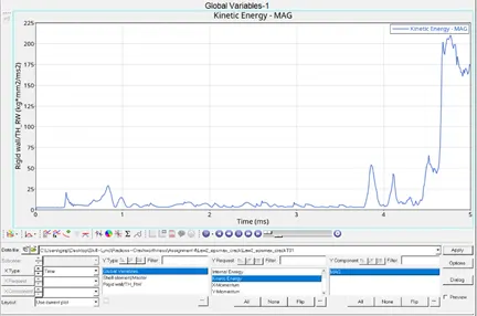
From the Internal energy curve, we can conclude that it reaches maximum energy nearer to 4.5ms which is later than when compared to the case1, also because of the crack propagation, Similar to kinetic energy.

3.Law2_epsmax_nofail

Import FAILURE_JOHNSON_0000.rad file in hypermesh(Solver Deck).

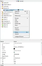
Delete the Failure_JOHNSON_1 card.

In Analysis panel, select Radioss and save the input file as Law2_epsmax_nofail_0000.rad in a separate folder (to save the animation files), mentioning the option = “-nt 4”.

Then run the input file, by selecting Radioss to perform the simulation.

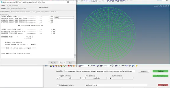
Select Results, to view the simulation – Select the Contour for displacement, von mises and save the files.

Go to Hypergraph, 2D to plot the desired graph for comparison.

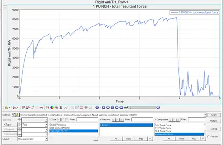
Total Resultant Force:

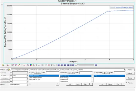
Internal Energy:

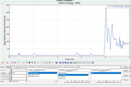
Kinetic Energy:

Total Energy:

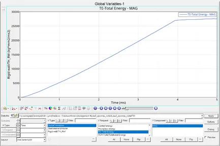
The component is now defined as elastoplastic material – having no failure, 15.1 % true plastic strain value.

Elements are getting deleted when strain – eps max is reached, which gives a linear increase in internal and total energy curves. Also, there is fluctuation in the Rigid Wall force around 4 ms, Same as the Case1.

4.Law2

Import FAILURE_JOHNSON_0000.rad file in hypermesh(Solver Deck).

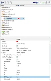
In Material, Aluminium – Delete the eps_p_max value i.e., = 0

In Analysis panel, select Radioss and save the input file as Law2_0000.rad in a separate folder (to save the animation files), mentioning the option = “-nt 4”.

Then run the input file, by selecting Radioss to perform the simulation.

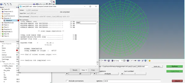
Select Results, to view the simulation – Select the Contour for displacement, von mises and save the files.

Go to Hypergraph, 2D to plot the desired graph for comparison.

Total Resultant Force:

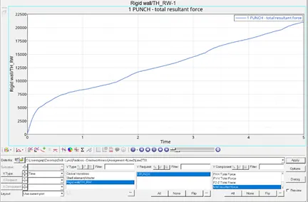
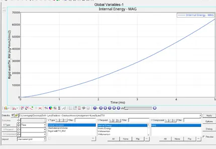
Internal Energy:

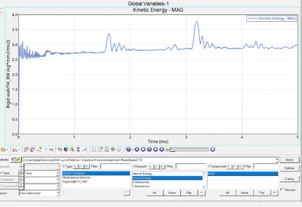
Kinetic Energy:

Total Energy:

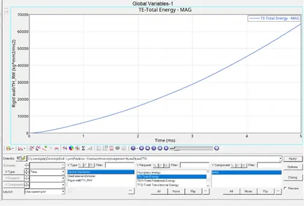
Element has no failure criteria since Failure Johnson & Eps max are deleted, i.e., default value 10³⁰

From the simulation, we can observe there is no deletion of elements and max von-mises stress.

Kinetic Energy reaches a maximum at the start since the failure happens only at the centre and propagates linearly.

5.Law1

Import FAILURE_JOHNSON_0000.rad file in hypermesh(Solver Deck).

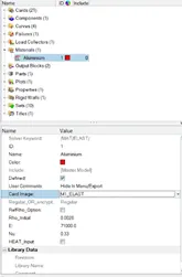
In Material, Aluminium – M1_Elast is selected for the card image and the following values are set.

In Analysis panel, select Radioss and save the input file as Law1_0000.rad in a separate folder (to save the animation files), mentioning the option = “-nt 4”.

Then run the input file, by selecting Radioss to perform the simulation.

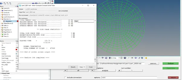
Select Results, to view the simulation – Select the Contour for displacement, von mises and save the files.

Go to Hypergraph, 2D to plot the desired graph for comparison.

Total Resultant Force:

Internal Energy:

Kinetic Energy:

Total Energy:

Component elements are defined as elastic - Law1 with density, E and nu, which gives linear towards stress and strain.

From the simulation, we can observe no elements got deleted. Also, the max of von mises strain is observed.

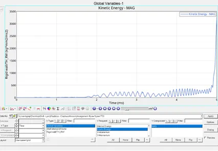
Kinetic Energy increases gradually and reaches maximum towards the end when maximum load is observed.

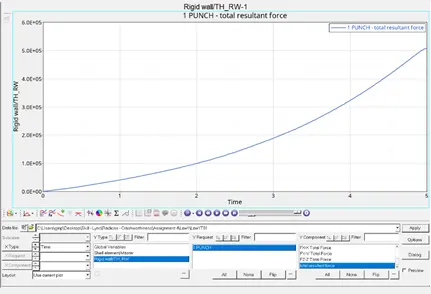
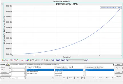
Internal energy & rigid forces increase exponentially due to the elastic nature of the elements, with no fluctuations.

6. Law27

Import Law27_0000.rad file in hypermesh(Solver Deck).

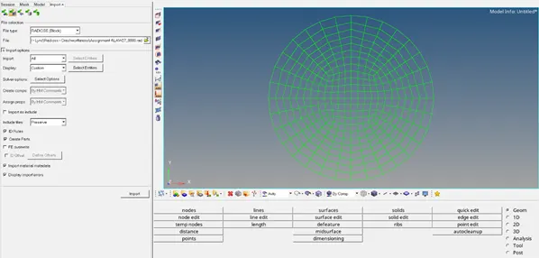
Change the shell properties as recommended in the Property Card of 5NiP as follows

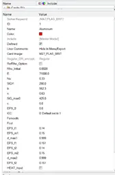
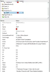
In Analysis panel, select Radioss and save the input file as Law27_0000.rad in a separate folder (to save the animation files), mentioning the option = “-nt 4”.

Then run the input file, by selecting Radioss to perform the simulation.

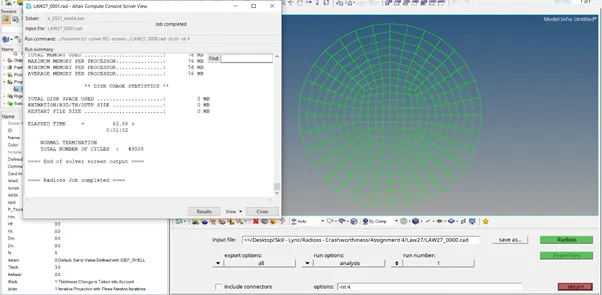
Select Results, to view the simulation – Select the Contour for displacement, von mises and save the files.

Go to Hypergraph, 2D to plot the desired graph for comparison.

Total Resultant Force:

Internal Energy:

Kinetic Energy:

Total Energy:

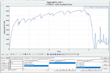
Elements are defined as isotropic elastoplastic Johnson-Cook material model, with orthotropic brittle failure model.

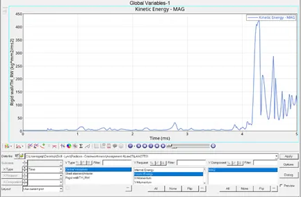
From the simulation, we can observe linear elastic when the element stress is lower than the plastic yield stress, higher values it is observed as plastic. Elements are deleted during maximum tensile strain during 4ms; material breaks like brittle at first.

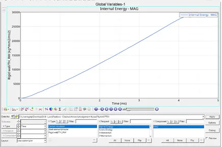
Internal energy increases linearly till 4ms, and reaches maximum due to element deletion, further it increases due to loss of strain energy from deleted/stressed elements.

7. Law36

Import Law27_0000.rad file in hypermesh(Solver Deck).

Create New Curve as follows

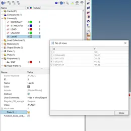
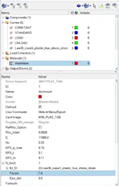
Set Values of Aluminium (Material) as follows (Change the card image – M36_PLAS_TAB)

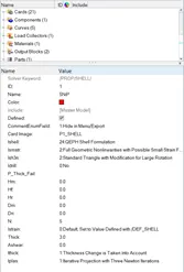
In Analysis panel, select Radioss and save the input file as Law36_0000.rad in a separate folder (to save the animation files), mentioning the option = “-nt 4”.

Then run the input file, by selecting Radioss to perform the simulation.

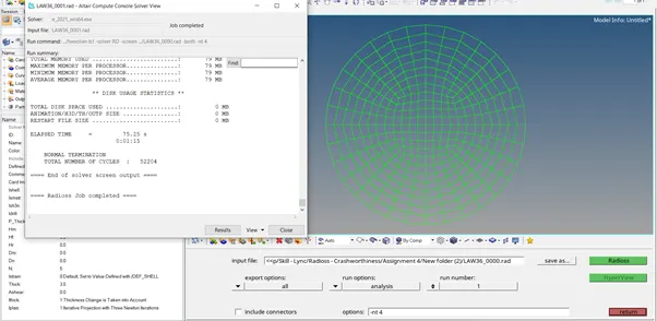
Select Results, to view the simulation – Select the Contour for displacement, von mises and save the files.

Go to Hypergraph, 2D to plot the desired graph for comparison.

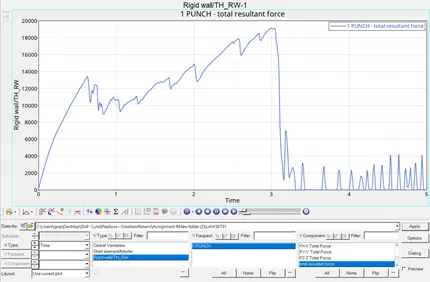
Total Resultant Force:

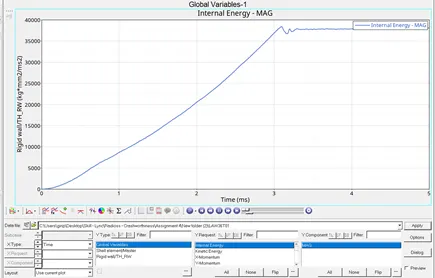
Internal Energy:

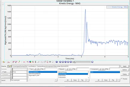
Kinetic Energy:

Total Energy:

Material Elements is defined as isotropic elastoplastic material with user-defined function of stress-strain curve (plastic true stress-strain)

From the Simulation, we can observe material is brittle and elements getting deleted from the centre completely.

	No. of Cycles	Energy error (%)	Mass Error	Simulation time (s)
Case 1 failure	49380	0.8	0	68.07
Case 2 crack	49217	4.1	0	133.30
Case 3 no-fail	49408	0.8	0	88.48
Case 4 Law 2	48737	3	0	91.48
Case 5 Law 1	47969	1.3	0	120.70
Case 6 Law 27	49508	0.8	0	62.88
Case 7 Law 36	52204	-1.7	0	75.25

Hour Glass Energy & Mass error is zero for all the cases.

No. of cycles is minimum for Law 1 as there are no elements to delete and maximum for Law 36 due to user-defined function to simulate.

Learning Outcome:

Law 1 - Elastic – Linear Stress-Strain curve

Law 2 - Linear Elastic up to yield stress value, then it is plastic

Law 27 - Brittle

Law 36 – Elastic-Plastic due to isotropic with the user-defined stress-strain curve.