Assignment 4-RADIOSS Material Laws Challenge

Objectives:-
To assign different material laws and properties to the given component and to compare their results and present the inference.

PROCEDURE:-

CASE 1:-

1.Go to FILE > IMPORT > SOLVER DECK > FAILURE_JOHNSON_0000.RAD > IMPORT. Then check the properties and change it to recommended properties if needed.
2.Now run the file. Go to ANALYSIS > RADIOSS > INPUT FILE > INCLUDE CONNECTOR > OPTIONS = -NT 4 > RADIOSS. Before running the simulation, change the file name to Law2_epsmax_failure_0000 and save it in a new folder.
3.Then run the simulation.
4.After running the simulation, open its .out file and note down the Total number of cycles, energy error, mass error and simulation time.
5.Now to view the animation, Open its .h3d file in hyperview and go to CONTOUR > RESULT TYPE > VON MISES > AVERAGING METHOD > SIMPLE > APPLY.
6.Then view the plot, open Hypergraph 2D and load its To1 file. Go to GLOBAL VARIABLES > INTERNAL ENEGRY, CONTACT ENERGY and TOTAL ENERGY > MAG > APPLY. This will plot the energy graph.

Results:-
1.In this case, the Law2 material card is used which represent the elasto-plastic material using the Johnson-Cook material model. This model expresses material stress as a function of strain, strain rate and temperature.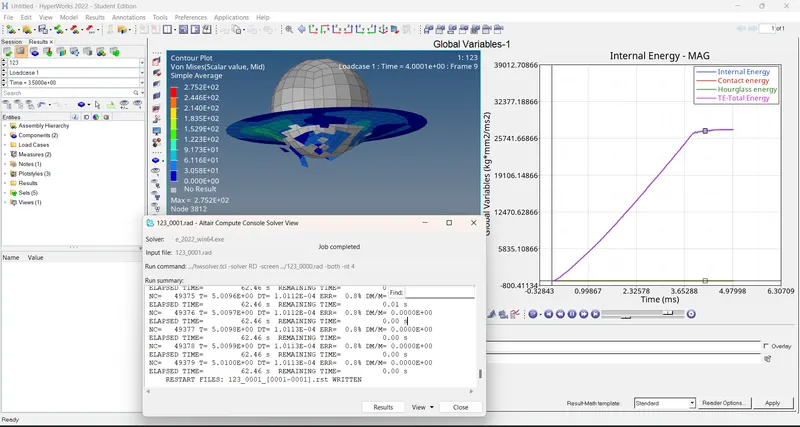
2.By Looking at the graph, the internal energy is high and hence the total energy is same as the internal energy. The total energy shows little variation from 4 ms.

CASE 2:-

1. Import the 'Law2_epsmax_failure_0000_RAD' file which was saved before.
2. After that, open the failures card and then open the Failure_JOHNSON_1 card under the failures card. And change Ifail_sh=1, Dadv = 1 and Ixfem = 1.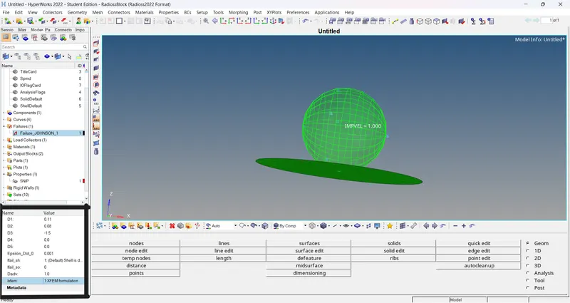
3. Now run the file. Go to ANALYSIS > RADIOSS > INPUT FILE > INCLUDE CONNECTOR > OPTIONS = -NT 4 > RADIOSS. Before running the simulation, change the file name to Law2_epsmax_crack_0000 and save it in a new folder.
4. Then run the simulation.
5. After running the simulation, open its .out file and note down the Total number of cycles, energy error, mass error and simulation time.
6. Now to view the animation, Open its .h3d file in hyperview and go to CONTOUR > RESULT TYPE > VON MISES > AVERAGING METHOD > SIMPLE > APPLY.
7. Then view the plot, open Hypergraph 2D and load its To1 file. Go to GLOBAL VARIABLES > INTERNAL ENEGRY, CONTACT ENERGY and TOTAL ENERGY > MAG > APPLY. This will plot the energy graph.

Results:-

1. We can observe the elements are getting cracked at initial stage. The cracking of elements is due to the Ixfem value set to 1. Ixfem =1 : failure element cracked. Ifail_sh =1: Shell element is deleted or craked when D = for one integration point or layer. Dadv = 1: max accumulation damage value D, used for crack initiation. (Criteria for crack advancement.)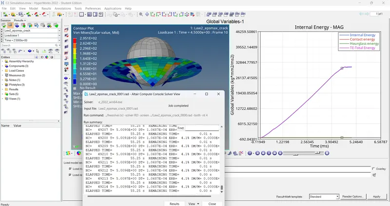
2. We can see that the internal energy is more than 30000 kgmm2/ms2 which is greater than the case 1. This is due to the elemens being deleted and the energy is stored as internal energy.

CASE 3:-

1.Import the 'Law2_epsmax_crack_0000.RAD' file which was saved before.
2.After that, Under the failures card, Delete the failure_JOHNSON_1 card by right clicking.
3.Now run the file. Go to ANALYSIS > RADIOSS > INPUT FILE > INCLUDE CONNECTOR > OPTIONS = -NT 4 > RADIOSS. Before running the simulation, change the file name to Law2_epsmax_nofail_0000 and save it in a new folder.
4.Then run the simulation.
5.After running the simulation, open its .out file and note down the Total number of cycles, energy error, mass error and simulation time.
6.Now to view the animation, Open its .h3d file in hyperview and go to CONTOUR > RESULT TYPE > VON MISES > AVERAGING METHOD > SIMPLE > APPLY.
7.Then view the plot, open Hypergraph 2D and load its To1 file. Go to GLOBAL VARIABLES > INTERNAL ENEGRY, CONTACT ENERGY and TOTAL ENERGY > MAG > APPLY. This will plot the energy graph.

Results:-
1.In this model there is no failure model, hence the material Law2 is obeyed.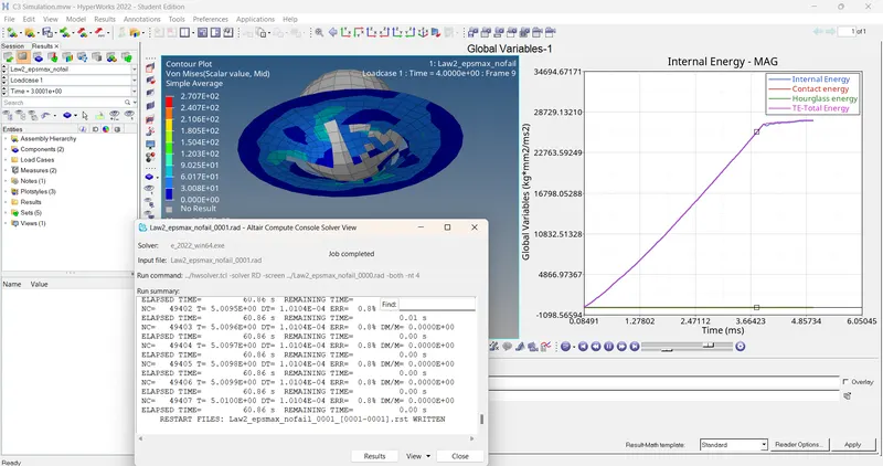
2.Here, the EPSmax value is followed for element failure.
3.We can observe the internal energy and the total energy curve follow same line until 4ms where the contact energy is constant.

CASE 4:-

1.Import the 'Law2_epsmax_nofail_0000.RAD' file which was saved before.
2.After that, Under the material card, click on the aluminium card and set hte EPS_P_MAX value to 0.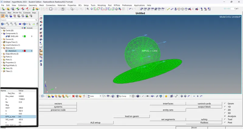
3.Now run the file. Go to ANALYSIS > RADIOSS > INPUT FILE > INCLUDE CONNECTOR > OPTIONS = -NT 4 > RADIOSS. Before running the simulation, change the file name to Law2_0000 and save it in a new folder.
4.Then run the simulation.
5.After running the simulation, open its .out file and note down the Total number of cycles, energy error, mass error and simulation time.
6.Now to view the animation, Open its .h3d file in hyperview and go to CONTOUR > RESULT TYPE > VON MISES > AVERAGING METHOD > SIMPLE > APPLY.
7.Then view the plot, open Hypergraph 2D and load its To1 file. Go to GLOBAL VARIABLES > INTERNAL ENEGRY, CONTACT ENERGY and TOTAL ENERGY > MAG > APPLY. This will plot the energy graph.

Results:-
1.Here the elements are being stretched like an elastic material. This is because the strain enters the plastic stage but as there is no eps_max value(set to zero), the Radioss will take the default value 103 which means that the material is not going to fail under plastic strain.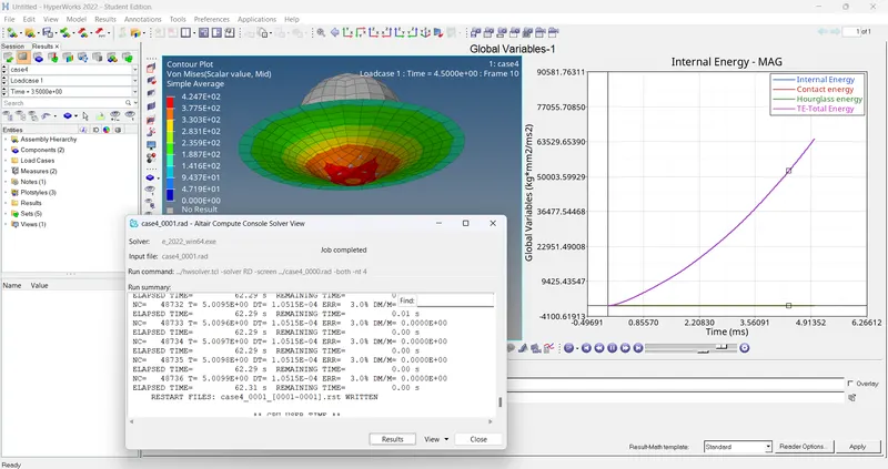
2.As compared to the case 3 energy curve we can see that case 4 energy curve shows more internal energy increasing at the end.

CASE 5:-

1.Import the 'case4_0000.RAD' file which was saved before.
2.After that, Go to the MATERIAL CARD > CARD IMAGE = M1 ELAST > Rho_initial = 0.0028, E = 71000 and Nu = 0.33. This will change the material properties from M2_PLAS_JOHNS_ZERIL to M1_ELAST.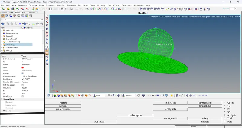
3.Now run the file. Go to ANALYSIS > RADIOSS > INPUT FILE > INCLUDE CONNECTOR > OPTIONS = -NT 4 > RADIOSS. Before running the simulation, change the file name to Law1_0000 and save it in a new folder.
4.Then run the simulation.
5.After running the simulation, open its .out file and note down the Total number of cycles, energy error, mass error and simulation time.
6.Now to view the animation, Open its .h3d file in hyperview and go to CONTOUR > RESULT TYPE > VON MISES > AVERAGING METHOD > SIMPLE > APPLY.
7.Then view the plot, open Hypergraph 2D and load its To1 file. Go to GLOBAL VARIABLES > INTERNAL ENEGRY, CONTACT ENERGY and TOTAL ENERGY > MAG > APPLY. This will plot the energy graph.

Results:
1.In this case, the plate component is defined as elastic material, hence the component will be in the elastic zone and will not enter the plastic deformation. Thus, there is no crack or element failure and maximum stress is developed at the contact between both the components.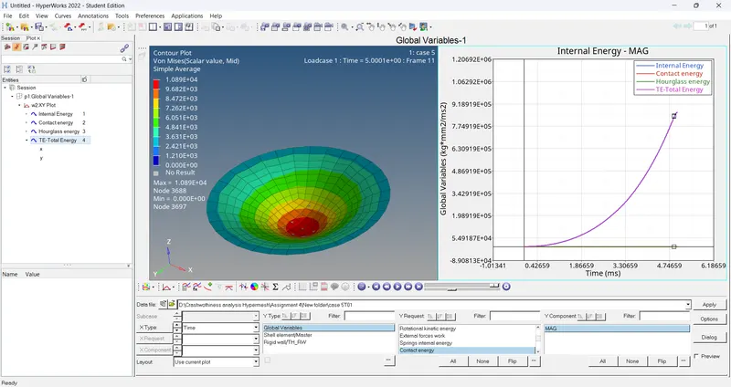
2.Though, we can see some elements penetrating through the plate elements, because the contact definition is not proper.
3.This curve shows more internal energy upto 800000 kgmm2/ms2 and contact energy is constant.

Case 6:-

1.Go to FILE > IMPORT > SOLVER DECK > Law2_epsmax_failure_0000.RAD > IMPORT.
2.Go to CURVES > CREATE > RENAME > PLASTIC_TRUE_STRESS_STRAIN_CURVE and enter the co-ordinates.
3.Go to MATERIALS > ALUMINIUM > CARD IMAGE = M36_PLAS_TAB.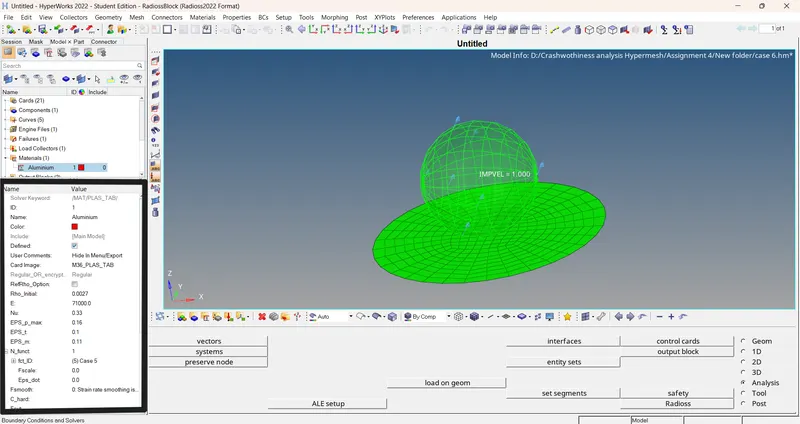
4.Now run the file. Go to ANALYSIS > RADIOSS > INPUT FILE > INCLUDE CONNECTOR > OPTIONS = -NT 4 > RADIOSS. Before running the simulation, change the file name to LAW_36_PLAS_TAB_0000 and save it in a new folder.
5.Then run the simulation.
6.After running the simulation, open its .out file and note down the Total number of cycles, energy error, mass error and simulation time.
7.Now to view the animation, Open its .h3d file in hyperview and go to CONTOUR > RESULT TYPE > VON MISES > AVERAGING METHOD > SIMPLE > APPLY.
8.Then view the plot, open Hypergraph 2D and load its To1 file. Go to GLOBAL VARIABLES > INTERNAL ENEGRY, CONTACT ENERGY and TOTAL ENERGY > MAG > APPLY. This will plot the energy graph.

Results:-
1.The Law36 material law helps in modeling isotropic elasto-plastic material using user defined functions for the work hardening portion of the stress-strain curve for different strain rates. The curve is nothing but the stress-strain curve after the yield point. The yield point is set to 0.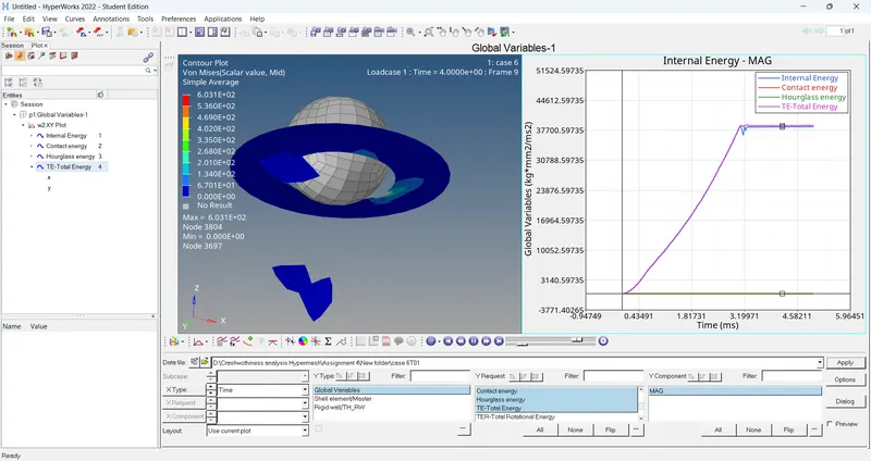
2.We observe that the elements fail at the maximum stress value and some elements are being deleted once they reach the EPS_f value. This type of failure is a real life failure as we have defined a true stress-strain curve. These curves are obtained from lab testing of the components.
3.This graph shows energy lesss than 30000 kgmm2/ms2 as we have used plas_tab material.

CASE 7:-

1.Go to FILE > IMPORT > SOLVER DECK > LAW27_0000.RAD > IMPORT.
2.Go to the property card and change the values as Ishell = 24, Ismstr = 2, Ish3n = 2, N = 5, Ithick = 1, Iplas = 1.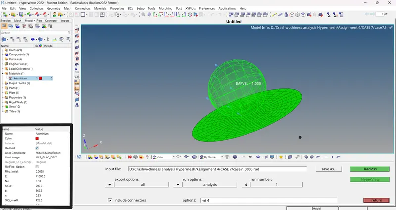
3.Now run the file. Go to ANALYSIS > RADIOSS > INPUT FILE > INCLUDE CONNECTOR > OPTIONS = -NT 4 > RADIOSS. Before running the simulation, change the file name to Law27_0000 and save it in a new folder.
4.Then run the simulation.
5.After running the simulation, open its .out file and note down the Total number of cycles, energy error, mass error and simulation time.
6.Now to view the animation, Open its .h3d file in hyperview and go to CONTOUR > RESULT TYPE > VON MISES > AVERAGING METHOD > SIMPLE > APPLY.
7.Then view the plot, open Hypergraph 2D and load its To1 file. Go to GLOBAL VARIABLES > INTERNAL ENEGRY, CONTACT ENERGY and TOTAL ENERGY > MAG > APPLY. This will plot the energy graph.

Results:-
1.In this case we use Law27 i.e. isotropic elasto-plastic material law with orthotropic brittle failure model. Orthotropic materials differ along three mutually-orthogonal axes. Here, the material damage and failure happens only in tension.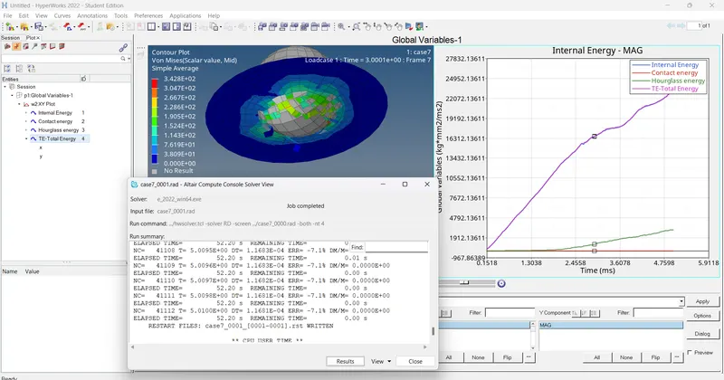
2.We can observe that some elements are failing like brittle material failure and also some elements being deleted.
3.This law allows the modeling of material damage and brittle failure in two principle directions which is controlled by EPS_f1 and EPS_f2.

Tabulated Data:-

CASES	Total No of Cycles	Energy Error	Mass Error	Simulation Time
CASE 1	49380	0.8 %	0	62.90
CASE 2	49217	4.1 %	0	55.25
CASE 3	49408	0.8 %	0	60.86
CASE 4	48736	3.0 %	0	62.31
CASE 5	47969	1.3 %	0	48.41
CASE 6	53144	-1.8 %	0	58.67
CASE 7	49508	0.8 %	0	53.91

Conclusion:-
Hence we conclude that the material laws and recommended properties have been applied and the results have been compared and inferred.