Assignment 4-RADIOSS Material Laws Challenge

Aim: To study the material laws and simulate the given model using objectives.

Objective: Perform the simulation as per the cases given below.

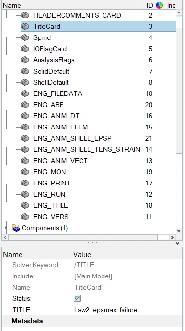
Case 1: Import the FAILURE_JOHNSON_0000.rad file and run the model as it is. Give the title name as Law2_epsmax_failure.

Case 2

• Import the case 1 rad file, named “Law2_epsmax_failure” and perform the simulation with failure plastic strain (EPS_p_max) and fail_Johson card enabled.
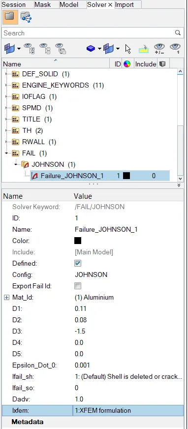
• Changes to be made in /FAIL/JOHNSON card:
• ifail_sh= 1
• Dadv= 1
• Ixfem= 1 
• Use the recommended values for the property card.
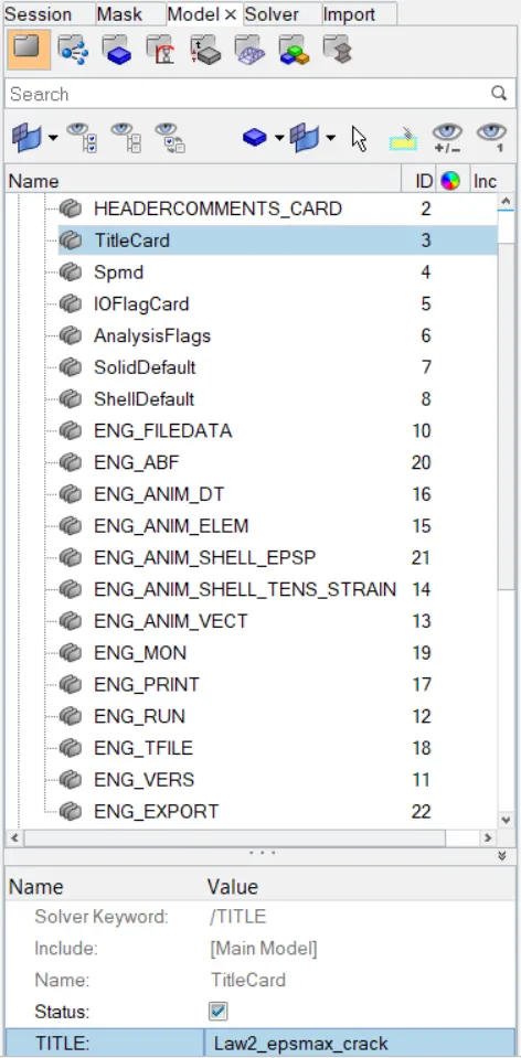
• Give the title name as Law2_epsmax_crack.

Case 3: Import the case 2 rad file, named “Law2_epsmax_crack” and perform the simulation by removing the fail_Johnson failure card. Give the title name as Law2_epsmax_nofail. 

Case 4: Import the case 3 rad file, named “Law2_epsmax_nofail” and perform the simulation by removing both the failure plastic strain (EPS_p_max) and the fail_Jhonson failure card.

Case 5: Import the case 4 rad file and perform the simulation by changing the material card to Law 1. Keep the same value for rho, E, and nu values.

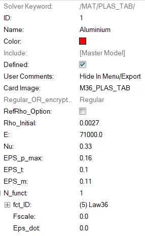
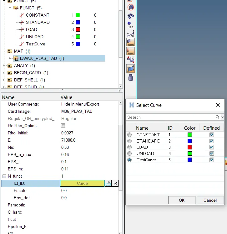
Case 6: Import the case 1 rad file, named “Law2_epsmax_failure” and perform the simulation with the law 36 material card.

 

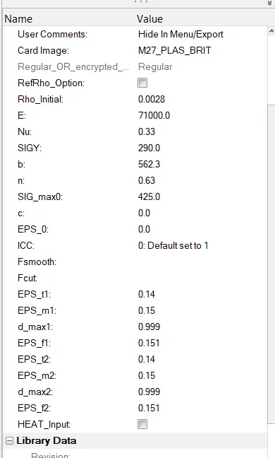
Case 7: Open the Law27_0000.rad file and perform the simulation with the law 27 material card. Use the recommended shell properties.    

Compare 7 cases as discussed in the last 3 slides, in a tabulated format based on:

1. The Total number of cycles, Energy error, mass error, and simulation time.
2. Notice the animation of all 5 and describe the animations in brief based on whether the elements are being deleted or cracked.
3. Plot energies and notice any difference.
4. Based on all the results, which case would represent the on-field scenario.
5. Prepare a ppt/Docx and list down case by case results and your conclusion as to why the failure happened.

Information:

The accuracy of the simulation depends on the material chosen. Choosing the right material and providing the reliable material data in performing a simulation is very important. RADIOSS has multiple material properties and wide variety of material library like concrete, foam, rubber, composites etc.,

Here in this challenge we have used 4 laws;

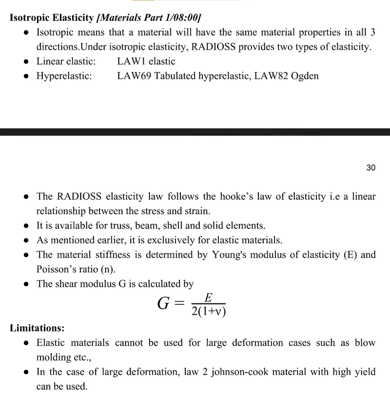
Law1: Elastic (Isotropic Elasticity)

This keyword defines an isotropic, linear elastic material using Hooke's law. This law represents a linear relationship between stress and strain. It is available for truss, beam (type 3 only), shell and solid elements. This material law is used to model purely elastic materials. The material stiffness is determined by only two values: the Young's modulus (E), and Poisson's ratio ( υ">υυ ). 

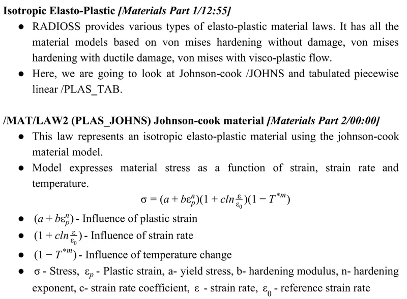
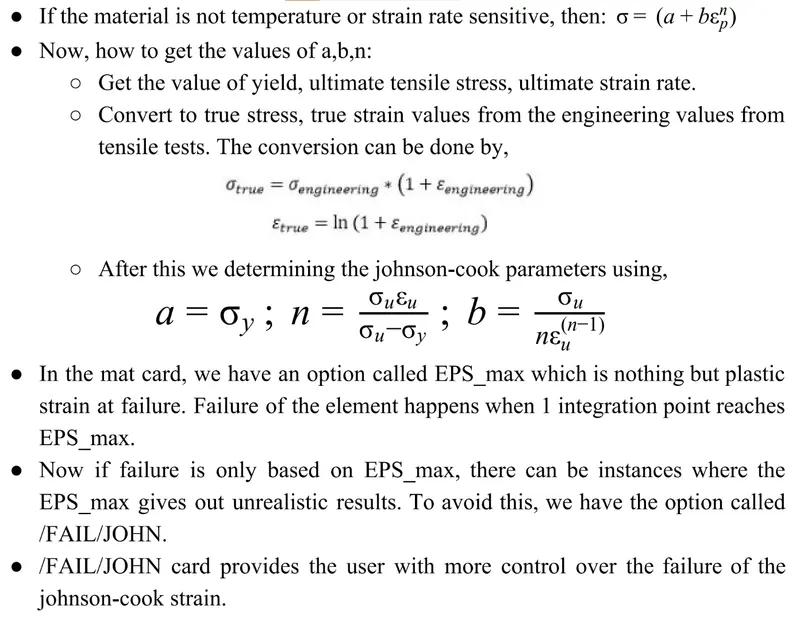
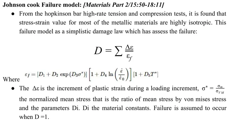
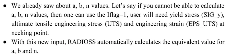
Law2: Johnson-cook (Isotropic Elasto-plastic)

This law represents an isotropic elasto-plastic material using the Johnson-Cook material model. This model expresses material stress as a function of strain, strain rate and temperature. A built-in failure criterion based on the maximum plastic strain is available. This is an elasto-plastic material model that includes strain rate and temperature effects with true stress and strain output. In this model the material behaves as a linear-elastic material when the equivalent stress is lower than the plastic yield stress. For higher stress values, the material behavior is plastic.

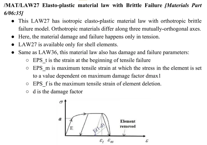
Law27: Elastic-plastic brittle

This law combines an isotropic elasto-plastic Johnson-Cook material model with an orthotropic brittle failure model. Material damage is accounted for prior to failure. Failure and damage occur only in tension. This law is applicable only for shells. 

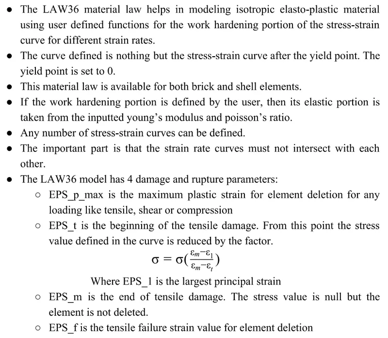
Law36: Elastic-plastic

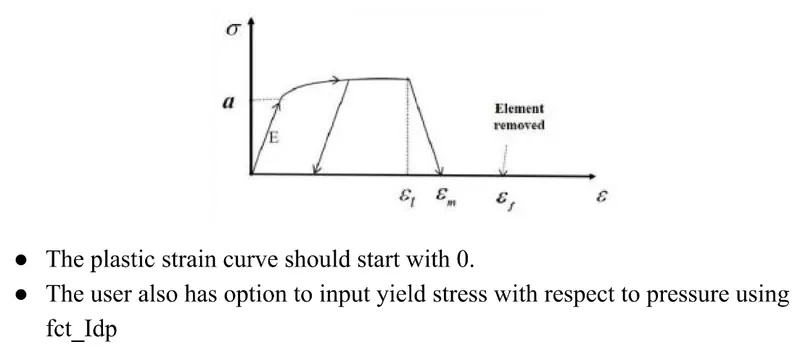
This law models an isotropic elasto-plastic material using user-defined functions for the work-hardening portion of the stress-strain curve (for example, stress versus plastic strain) for different strain rates.

Procedure:

For CASE 1:

First Import the file provided and change the title in the title card as shown below and run the file using analysis>radioss>filelocation>radioss.

For CASE 2:

Import the case 1 rad file, named “Law2_epsmax_failure” and perform the simulation with failure plastic strain (EPS_p_max) and fail_Johson card enabled with following inputs as shown and run the analysis:

For Case 3:

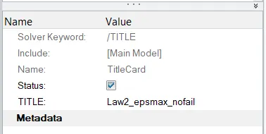
Import the case 2 rad file, named “Law2_epsmax_crack” and perform the simulation by deleting/removing the fail_Johnson failure card and give the title name as Law2_epsmax_nofail and run the analysis.

For Case 4:

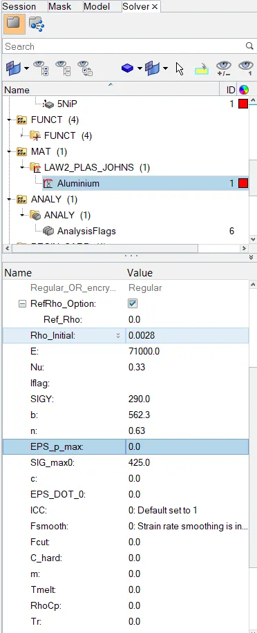
Import the case 3 rad file, named “Law2_epsmax_nofail” and perform the simulation by removing both the failure plastic strain (EPS_p_max) and run the analysis.

.

For Case 5: Import the case 4 rad file and perform the simulation by changing the material card to Law 1; keep the same value for rho, E, and nu values and run the analysis.

From 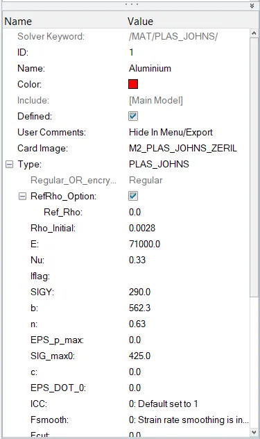to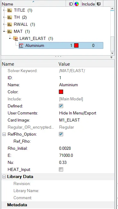

For Case 6:

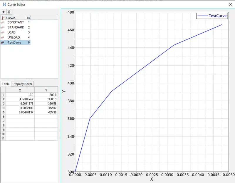
Import the case 1 rad file, named “Law2_epsmax_failure” and perform the simulation with the law 36 material card and run the analysis. Create a stress strain test curve as shown below:

For Case 7:

Importing Law27_0000.rad file and perform the simulation with the law 27 material card using the recommended shell properties.

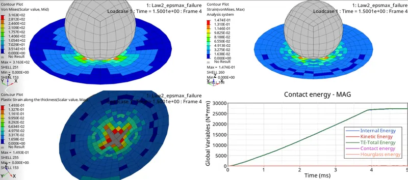
• Now, we divide the graphics window into 4 parts and after running all the analysis, and use 3 windows to open the h3d file and 1 window for T01 file. We now get the following results as shown below:

For CASE 1:

For CASE 2:

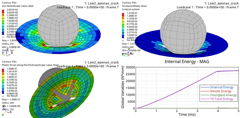
For CASE 3:

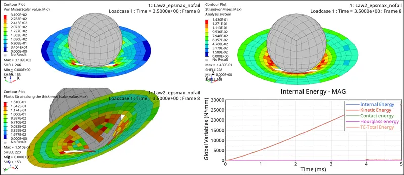
For CASE 4:

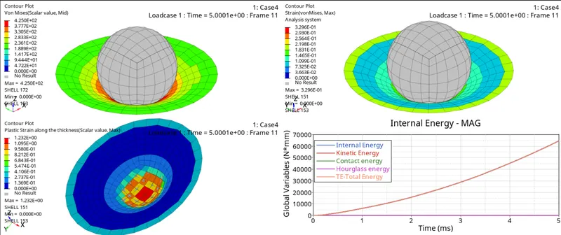
For CASE 5:

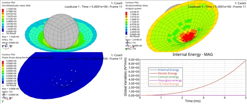
For CASE 6:

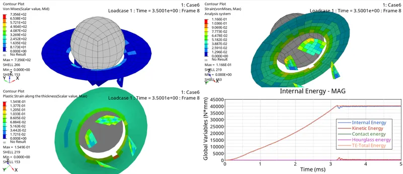
For CASE 7:

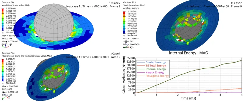
Observation:

When can we say that the element has been deleted? - Just by observing the animations we cannot say that the elements have been deleted, so here comes the role of the graphs. When there is a slight dip in the curve of internal energy then we can say that the elements have been deleted or cracked or there is no interaction between them because when the element is stretched then there is an internal energy developed in elements. If any element is deleted then there will be a decrease in the internal energy. In elastic the elements will not be deleted or cracked and will keep on absorbing the energy which implies that the energy will be constant.

• As we can observe in the graphs above for all the cases, we can say that the internal energy for case 4 and case 5 keep on increasing. Also, in animations the surface is intact and not shearing apart which means that the . So, we reject the cases 4 and 5.
• For case 7, by observing the graphs and animations the elements energy is increasing and also there is no drop in it which means that case 7 can be represented or used for a particular scenario but it is a brittle material and the energy error is also -7.1 %.
• For case 1, 2, 3 and 6; after a linear increase there is a dip in the internal energy which means that the elements are deleted or cracked which is not suitable for any real life scenario.

Conclusion:

• Checking .out file for the output results:

Now let us open the 0001.out file using notepad for simulation time, number of cycles, energy error, kinetic energy, internal energy and mass error.

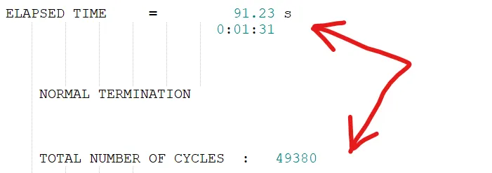
Similarily, we check for all the cases and get the following results as shown in the conclusion:

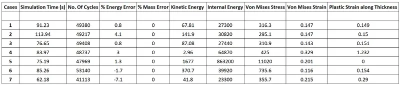
From all the cases or the three laws used, law2 and law 27 both use johnson cook to describe the elasto plastic behaviour i.e. law2 with plastic strain and law27 with principal strain. Here, 6th case with law36 seems to be more realistic since we have manually added the real life stress strain curve data where the material is behaving according to it. Due to this it has maximum number of cycles and takes more time when compared with most of the cases; the energy error is -1.7% which is in the range.