Assignment 4-RADIOSS Material Laws Challenge

1. Introduction

Radioss is a widely used solver known for its ability to solve explicit dynamic problems such as crash simulations. There are a number of material models available in the solver that can be used for modelling materials with the best possible description.

There are a number of material models used for modelling commonly used metals and alloys in engineering. Some of them are shown in the below-attached figure.

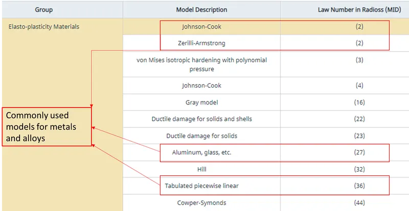
Fig 1.1: Different material models for the elastic-plastic type of behaviour

Other than these models there are numerous other models suitable for different kinds of behaviours. For example materials such as rubbers can be modelled using hyperelastic material models like the Ogden material model which takes care of material behaviour based on strain energy.

In this exercise, three elastic-plastic material models were used in a plate rupture model along with certain failure criteria. The mode of element failure was compared for different materials. The unit system followed in the exercise is [g-mm-ms].

2. The Model

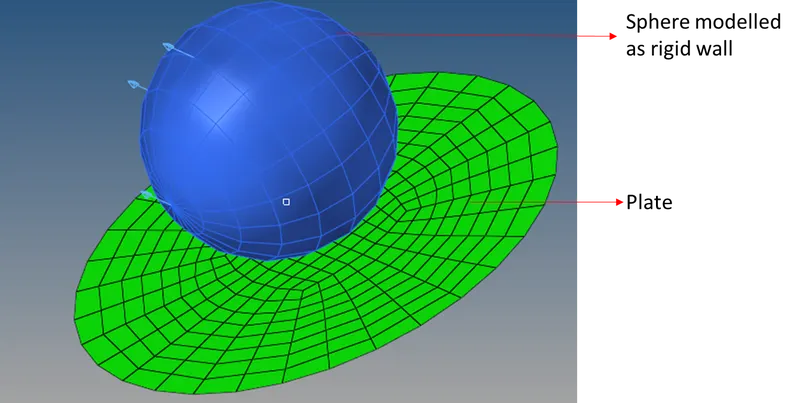
Fig 2.1: The geometry used in the model

As shown in the above figure, the geometry consists of a circular plate meshed with shell elements and a sphere modelled as a rigid wall. A thickness of 3 mm was used for the plate and all the shell properties were assigned case by case which will be discussed separately. Further, the following boundary conditions were used:

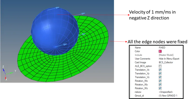
Fig 2.2: The boundary conditions applied to the model

These two boundary conditions were able to allow the ball to rupture the plate and cause the element to fail. Apart from this, all other necessary cards were added like Run was used to define a termination time of 5 ms and anim dt was used to request animation files for every 0.1ms.

A number of cases were simulated to examine the failure of elements when modelled with different material laws and failure criteria. The cases are shown in the below-attached figure:

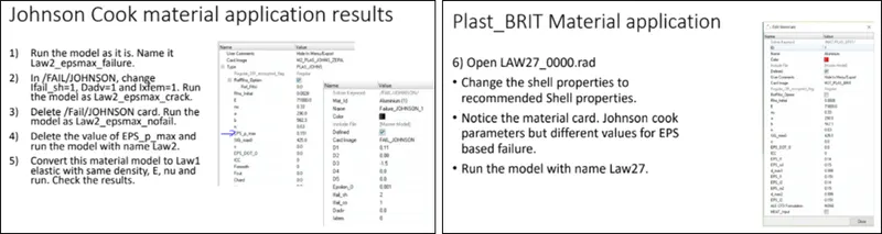
Fig 2.3: The cases simulated for this exercise

3. Case 1: Material model- Law 2 Johnson-Cook Elasto-plastic

This card is used for modelling commonly used metals and alloys that exhibit elastoplastic behaviour, especially ductile metals. Properties of Aluminum was used with the [gm-mm-ms] unit system. The material card is shown in the attached figure.

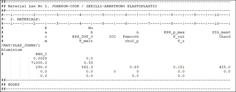
Fig 3.1: The material card used for the model

This law represents an isotropic elastoplastic material using the Johnson-Cook material model. This model expresses material stress as a function of strain, strain rate and temperature. A built-in failure criterion based on the maximum plastic strain is available. In this model, the material behaves as a linear-elastic material when the equivalent stress is lower than the plastic yield stress. For higher stress values, the material behaviour is plastic, and the true stress is calculated as:

`sigma = (a+b.epsilon_p^n)(1+c ln(epsilon^./epsilon_o^.))*(1-T^*m)`

Where `sigma` = stress, `epsilon_p` = plastic strain, a= Yield stress, b= hardening modulus, n= hardening exponent, c= strain rate, `epsilon^.`= strain rate, `epsilon_o^.` = reference strain rate.

In this model a failure Johnson card as shown in the attached figure was used with the Ifail sh set to 2 which means for each integration point, the stress tensor is set to zero when `D=∑Δε_pε_f≥1"`. The shell is deleted or cracked when `D=∑Δε_pε_f≥1"` for all integration points or layers. Results are discussed in the below section:

3.1 Results and discussion

Animation 3.1: The failure of the elements using EPS max value

As clear from the animation, the elements at the bottom are getting deleted. The failure must be happening based on the values of parameters D1-D5 in the failure card. The Johnson Failure card is discussed in section 4.

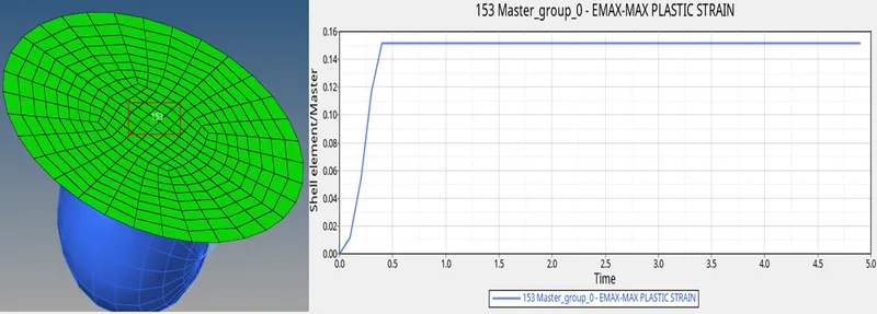
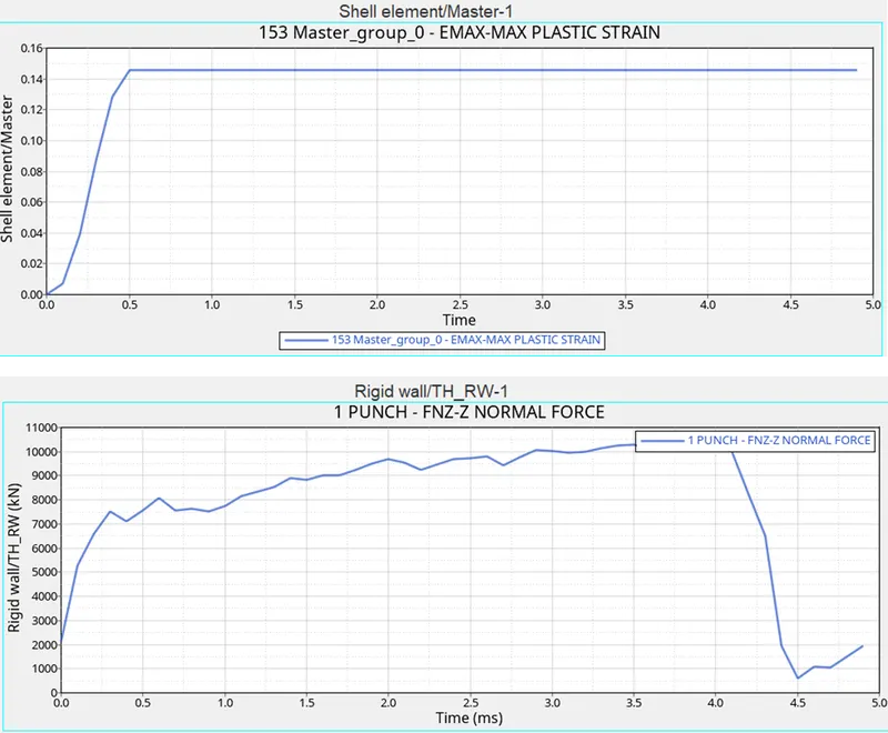
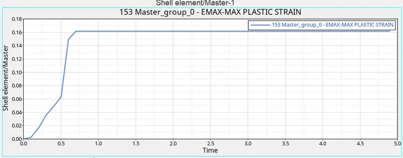
Fig 3.1.1: the EPS vs time plot for the element number 153

As clear from the plot, the max value attained in the element is close to the EPS max value of 0.151 which supports our theory. Next, we need to examine the energy plots so that we can confirm whether the simulation went well or there were some errors.

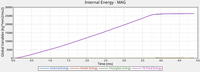
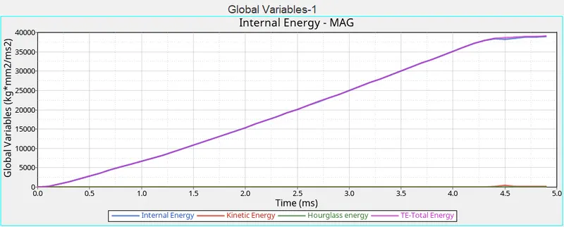
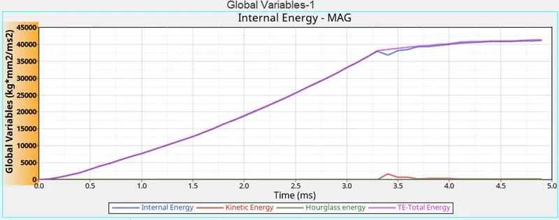
Fig 3.1.2: The energy plots for the model

The energy plots clearly suggest the addition of external work leads to the generation of strain energy and ultimately the internal energy goes up. Further, the kinetic energy is very low as the gap between the plate and punch is kept very little, this leads to the total energy almost following the internal energy as [T.E= I.E+K.E]. Also, the hourglass energy is very low which rules out the presence of any error due to the hourglass effect.

One more set of checks we need to perform is the check for energy error and mass error in the 001.out file. This tells us whether the simulation method adopted was reliable or it could have been better. Basically, the energy error must be negative and decreasing (except for the first cycle or in a spring back stage). The error must be less than 15% at the end of the computation (5% for a good model).

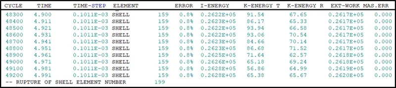
Fig 3.1.3: the snapshot from .out file of the simulation

As clear from the above figure, the energy error is very low and mass error is zero. which tells us that the simulation was ok.

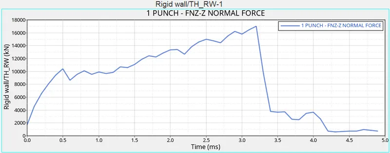
Next, we can plot the rigid wall forces as well for the model. This can be done from the Hypergraph by selecting the

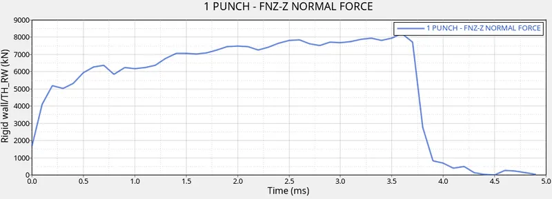
Fig 3.1.4: The plot of the normal force in the Z direction on the rigid wall

The above plot clearly tells the rupture that happened between 3.55 and 4.0 ms after which the force came down almost to zero. This is in agreement with the other conclusions.

4. Case 2: Using the /Fail/Johnson card for defining failure criteria in the Johnson cook material model

This time a failure card was added to the model as shown in the attached figure.

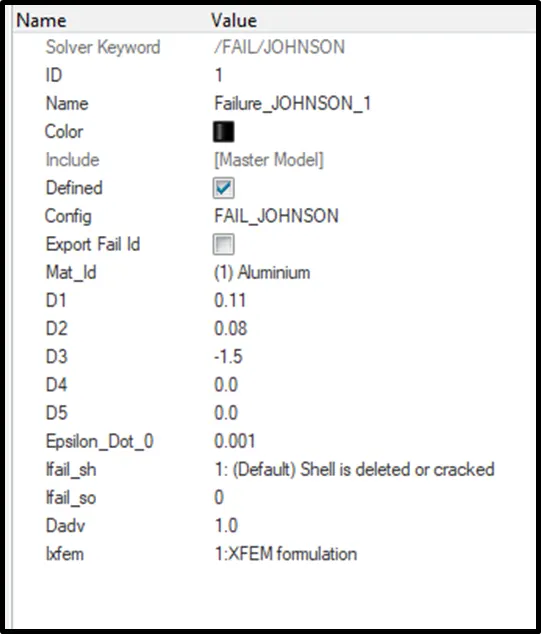
Fig 4.1: the failure Johnson card

The parameters D1 to D5 needs to be obtained using a number of iterations and typically they are provided to the modeller. The calculation is shown in the below snapshot.

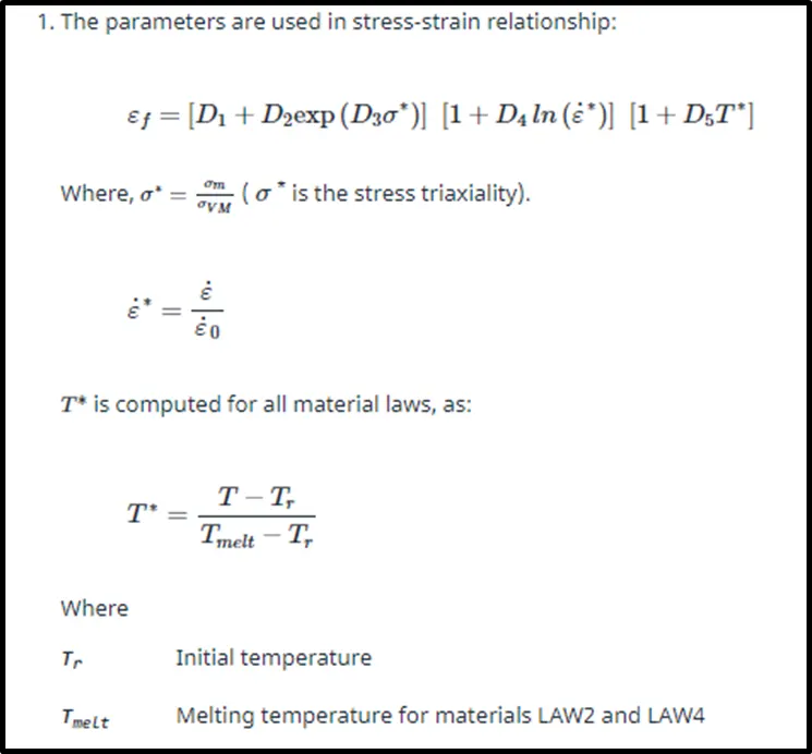
Fig 4.2: The calculation for Parameters D1 to D5

In the above figure, `epsilon_f` is the failure strain where the element is deleted during simulation. The Ifail sh was changed to 1, which means the failure will be captured by both deletion or cracking of the element where strain value reaches the failure point. Also, the IXFEM was changed to 1 meaning we want the failed element to crack rather than getting simply deleted. The material model needs to be very accurate for this to work properly.

All other things were kept unchanged and the simulation was run.

Anim 4.1: The cracking of elements

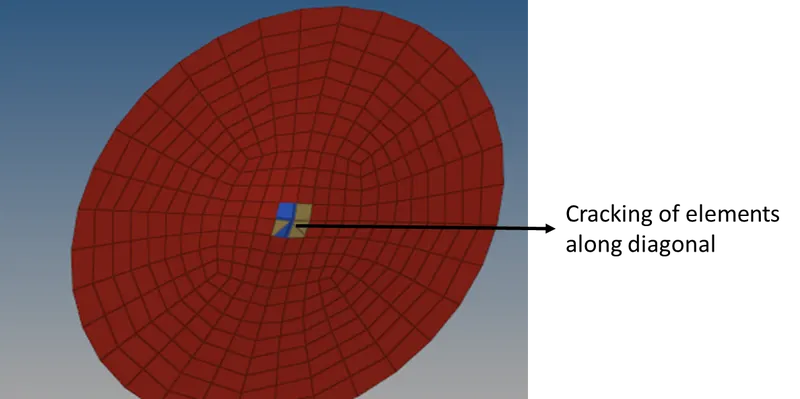
Fig 4.3: The initiation of a crack in the elements

Clearly, the failure was happening by cracking of the elements in the model upon reaching the failure point based on the criteria.

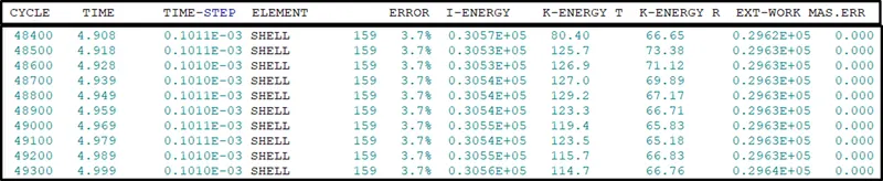
Fig 4.4: The snapshot from the .out file

This time the added energy goes up to 3.7% whereas the masses addition remains zero. This is an indication that with failure cards additional damping cards like hourglass control needs to be used to keep the energy error within the check. This bounce in energy error can be attributed to the fact that this time several cracked elements get deleted together unlike the deletion in the previous case.

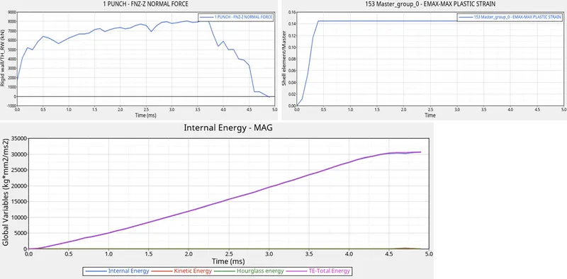
Fig 4.5: the different plots for the model

All the curves are similar in nature without any significant deviation from the earlier case. So all the previous explanations hold good for these curves too.

5. Case 3: Delete the /Fail/Johnson card and run the model

This time the Fail johnson card was deleted from the model and the failure now will be controlled by the EPS value in the elements.

Animation: The failure of elements

The animation clearly shows elements were deleted after reaching the limit values of EPS. The failure mode is similar to case 1. also, the energy error and mass addition were the same as in case 1.

6. Case 4: Delete the value of EPS max and run the model

This time the /Fail/Johnson card was deleted and also EPS max value was deleted. This leads to the failure being governed by the default value for eps max. The default value is 10^30 according to the manual, which is not possible to achieve in reality. This leads to continuous deformation of the pate without rupture as seen in the below-attached animation.

Animation: The simulation with the material without failure

This result is totally unrealistic and the simulation is going to fail if the run time is increased. Also the energy error this time jumps to 3.0% which makes it an inferior idea as compared to the above case.

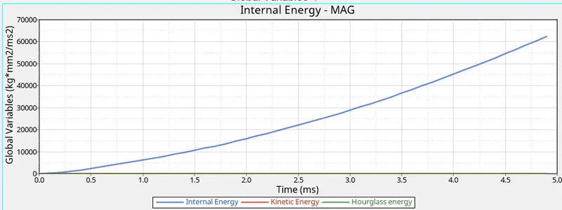
Fig 6.1: The energy plot for the material model without failure

The energy I.E. and total energy are increasing in an exponential form throughout the simulation. This does not match with the earlier cases as there is no break in the curve due to the absence of element failure.

7. Case 5: Convert this material data to law 1 elastic material model and check the results

In this case, the elastic material model (law1) was used to model the same material with elastic behaviour. The values of density, Young's modulus and Poisson's ratio were used from the material data.

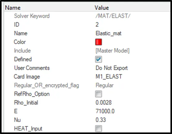
Fig 7.1: The elastic material card used for the model

Further, all other settings were kept the same and the simulation was run. The results are discussed below.

Animation: Simulation with the elastic material model

As clear from the animation, the material goes on stretching in an elastic manner, however, the jerks can be visualised in the punch. This can be due to elastic recoveries from the elements of the area surrounding the contact point.

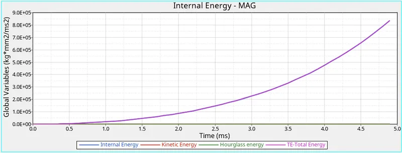
Fig 7.2: The plot of energies for the model

The plot resembles the energy curve for the previous case where there was no failing element and all the external work was getting added as internal energy.

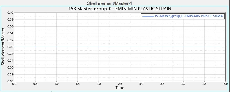
Fig 7.3: The plot of EPS for the element 153

As clear from the above plot the elements were behaving in the perfect plastic manner without any plastic strain. This is a result of the elastic material model used for the plate. The energy error, in this case, was 1.6% in the last step.

8. Case 6: Use the Law 27 material model for the simulation

This law is present by the name of Brittle Damage: Johnson-Cook Plasticity Model (LAW27). Johnson-Cook plasticity model is presented in the Johnson-Cook material model. For shell applications, a simple damage model can be associated with this law to take into account the brittle failure. The crack propagation occurs in the plan of shell in the case of mono-layer property and through the thickness if a multi-layer property is defined.

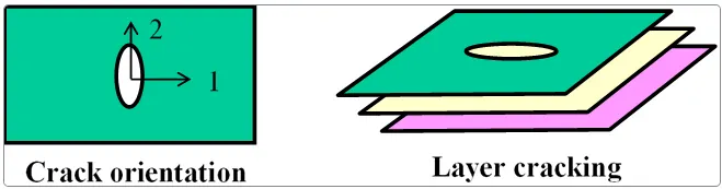
Fig 8.1: the damage modelled as a crack in single layer shell and multi-layer shell

The elastic-plastic behaviour of the material is defined by the Johnson-Cook model. However, the stress-strain curve for the material incorporates a last part related to the damage phase.

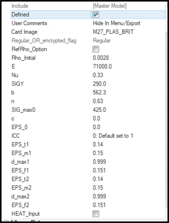
Fig 8.2: The Law 27 Card

AS seen in the card a number of parameters need to be defined for the model. Some of them are explained below:

1. Case 4 in which there were no failure criteria defined even though Law 2 card was used, gives the most unrealistic result and should not be preferred if the choice is available.
2. An elastic model should not be used for components where permanent deformation or failure is expected.
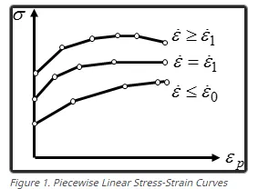
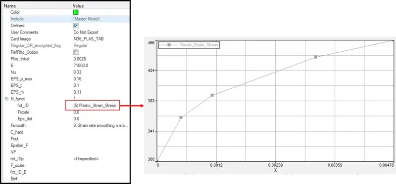
3. A choice between Law2 and LAw 36 needs to be made: Law 36 require the plastic stress-strain data and gives a more accurate behaviour while the law2 is simple in comparison to law 36.
4. Law 27 can be used for components where damage is expected in the form of cracks.