Assignment 4-RADIOSS Material Laws Challenge
AIM:
To simulate the crash analysis on the given model by applying different materials laws avaliable in Radioss.
OBJECTIVE:
1.To carry out the simulations of the given starter files and compare the results.
2.The file to be worked on are the FAILURE_JOHNSON_0000.rad file and the LAW27_0000.rad file.
3.Listed below are the cases as follows:
I)Law 2- FILE NAME: FAILURE_JOHNSON_0000.rad - Base Simulation.
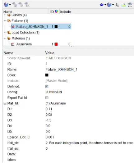
II)Law 2 - FILE NAME: FAILURE_JOHNSON_0000.rad - Ifail_sh =1, Dadv =1, Ixfem =1.
III)Law 2 - FILE NAME: Starter file for case 2 - fail card are deleted.
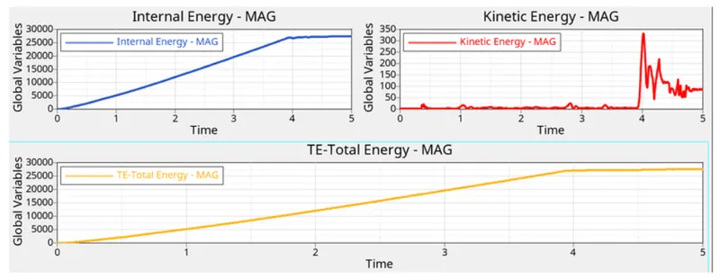
IV)Law 2 - FILE NAME: Starter file for case 3 - EPS_p_max value deleted.
V)Law 1 - FILE NAME: FAILURE_JOHNSON_0000.rad - fail card deleted and values for density, E, nu is assigned.
VI)Law27 - FILE NAME: LAW27_0000.rad - recommended shell properties is assigned.
VII)Law 36 - FILE NAME: LAW27_0000.rad - recommended shell properties and given reference curve is assigned.
THEORY:
1.The accuracy of the simulation depends on the material choosen.
2.Choosing the right material and providing the reliable material data in performing a simulation is important.
3.RADIOSS has multiple material properties and wide variety of material library like concrete, foam, rubber etc...
4.Some of the commercially used material laws are:
I)Law 1: Elastic(Isotropic Elasticity).
II)Law 2: Johnson-cook(Isotropic Elasto- Plastic).
III)Law27: Elastic-Plastic Brittle.
IV)Law36: Elastic-Plastic Tabulated.
V)Law42: Ogden(Visco Hyperlastic).
VI)Law70: Foam.
ISOTROPIC ELASTICITY-LAW 1:
Isotropic means that a material will have the same material properties in all 3 directions. Under isotropic elasticity, RADIOSS provides two types of elasticity.
1.Linear Elastic: LAW1 elastic
2.Hyper Elastic: LAW69 Tabulated hyperelastic, LAW82 Ogden.
The RADIOSS elasticity law follows the hook's law of elasticity i.e a linear relationship between the stress and strain. It available for truss, beam, shell and solid elemements. It is exclusively for elastic materials. The material stiffness is determined by Young's Modulus of Elasticity(E) and Poisson's Ratio(n).
The sheer modulus G is calculated by,
G = E / 2(1+V).
ISOTROPIC ELASTO-PLASTIC:
RADIOSS provides various types of elasto-plastic material laws. It has all the material models based on von mises hardening without damage, von mises haedening with ductile damage, von mises with visco-plastic flow.
Johnson-cook material(PLAS_JOHNS) - Law2:
This law represents an isotropic elasto-plastic material using the johnson-cook material model. The model expresses material stress as a function of strain, strain rate, and temperature. In the material card we have an option called EPS_max which is plastic strain at failure. Failure of the element happens when 1 integration point reaches EPS_max.
Now if failure is only based on EPS_max there can be instances where the EPS_max gives out unrealistic results. To avoid this we have the option called /FAILS/JOHN. This card provides the user with more control over the failure of the johnson-cook strain.
LAW36-PLAS_TAB Elastic Plastic Piecewise Linear Material:
The LAW36 material law helps in modeling isotropic elasto-plastic material using user defined functions for the work hardening portion of the stress-strain curve of different strain rates. The curve defined is nothing but the stress-strain curve for different strain rates. The curve defined is nothing but the stress-strain curve after the yield point. The yield point is set to 0.
The material law is avaliable for both brick and shell elements. If the work hardening portion is defined by user then its elastic portion is taken from the inputted young's modulus and poisson's ratio. Any number of stress-strain curves can be defined. The important part is that the strain rate curves must not intersect with each other.
The plastic strain curve should start with 0. The user also has option to input yield stress with respect to pressure using fct_Idp.
PROCEDURE:
CASE-1:
1.Import the model.The FAILURE_JOHNSON_0000.rad is selected and imported.
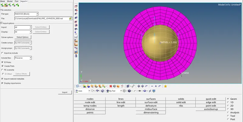
2.For this basic simulation, we will run the simulation with the default values.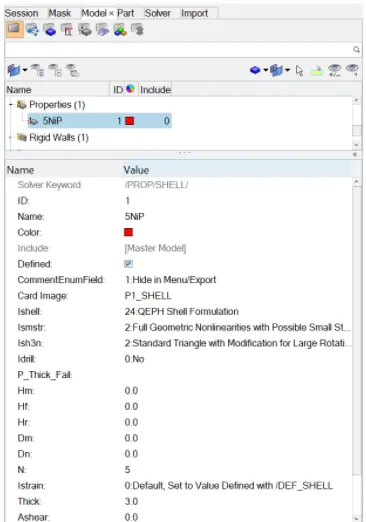
3.To run the simulation, Goto Analysis > RADIOSS. We need to save the output files in a new folder so that we can access them easily. The file is saved.
4.After saving, tick the include connectors box and type in -nt 4 in the options.
5.-nt 4 means assigning the task to 4 cores in the system to perform the simulation faster. It depends upon the process of our computer. And nt means number of threads. Then click on RADIOSS in order to run the simulation.

6.By clicking RADIOSS we get the solver window which basically shows us what the RADIOSS solver is done.
7.The simulation is complete. To view the result we need to switch to the Hyper utility.
8.After accessing Hyperview, we should input the simulation file. For this used h3hd file that was generated when RADIOSS processes the starter file. It is generated in the files. After selecting it click apply.
9.It generates the simulation animation.
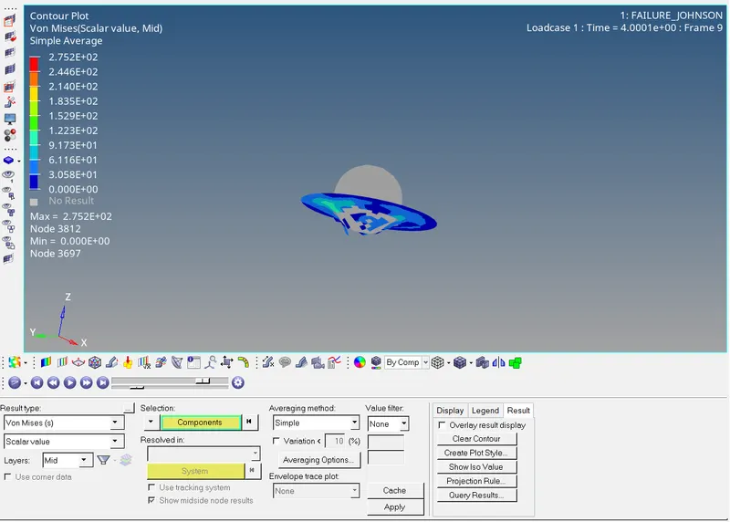
10.We can change what is being represented by selecting the contour option in the toolbar. We can change the result type to Von Mises and change averaging method to simple. Doing so creates the Von Mises stress contour is attached in given below section as Case-1.
11.Next is to carry out energy error and mass error checks and this is done by analyzing the RADIOSS engine output file. This can be accessed from the same directory as the starter and engine files and is denoted by the .out extansion.
12.We need to check the file that contains _0001.out by using text editor.
13.The final energy error is 0.8% which is acceptable. The closer to 0 it is the better and there is no mmass error.
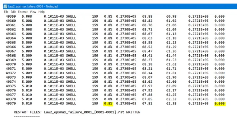
14.The highlighted potion are the end result.
15.Now plot the graphs in HyperGraph 2D. We can switch to it using the same client selector option in the toolbar.
16.In Hypergraph section, we need to input a file. We will be using the result file generated by the RADIOSS solver.
17.The file is avaliable in the same directory as the starter, engine, and animation files. The file name end with T01.
GRAPHS:
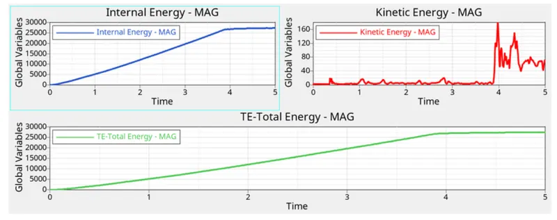
18.It has the Fail/JOHNSON card as well as EPS_p_max value assigned with Ixfem values as 0. This means that the elements are deleted as soon as they cross the EPS_p_max threshold.
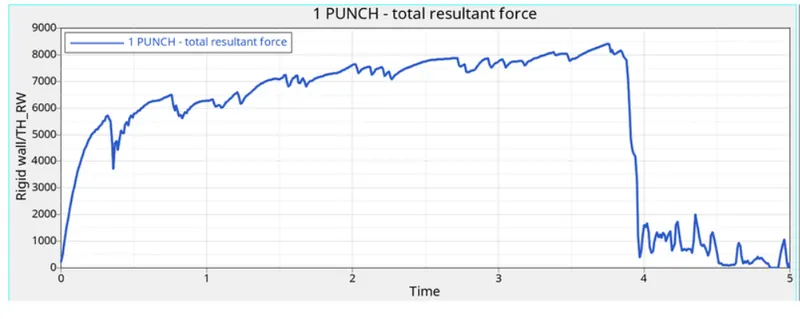
19.Internal energy as well as rigid wall forces are reactions to the force generated by the sphere on the sheet. Energy increases linearly until many elements are deleted at around the 4m/s threshold.
20.This creates vibration and that results in a surge of kinetic energy at the same point.
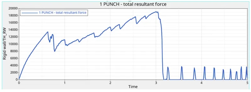
21.The rigid wall forces fluctuate when the elements are deleted and when a large chunk of elements are deleted at 4m/s. the graph drops meaning there are not many elements opposing the force of the sphere. Most of the elements in its path have been deleted at that point.
CASE-2:
1.Import the model.The FAILURE_JOHNSON_0000.rad is selected and imported.
2.We make some changes to the fail card. It can be accessed via the model tab.
3.Ifail = 1, determines the shell element failure method. So there are two ways in which we can see the element failing.
3.The element will either get deleted or in some cases the craking occurs according to the material properties.
4.In Ixfem, we can choose that if there is any element that is failing we want that element to delete or we want the element to be cracak.
5.We are going to take Ixfem =1. Which allows failed element to cracked not to delete.
6.In Dadv, we take Dadv =1. Which gives the criteria that how much an element can get break into small pieces. If it goes beyond the limit the element gets deleted.
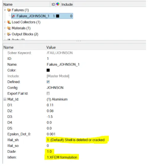
7.The highlighted region are the changed properties.
8.Now run the analysis and the file is saved and -nt 4 typed in the options box we can click the RADIOSS button to run the analysis.
9.After the solver window completes the analysis as usual switch to Hyperview window and run the h3d file of the current analysis and set the Von Mises stress contours is attached in given below section as Case-2.
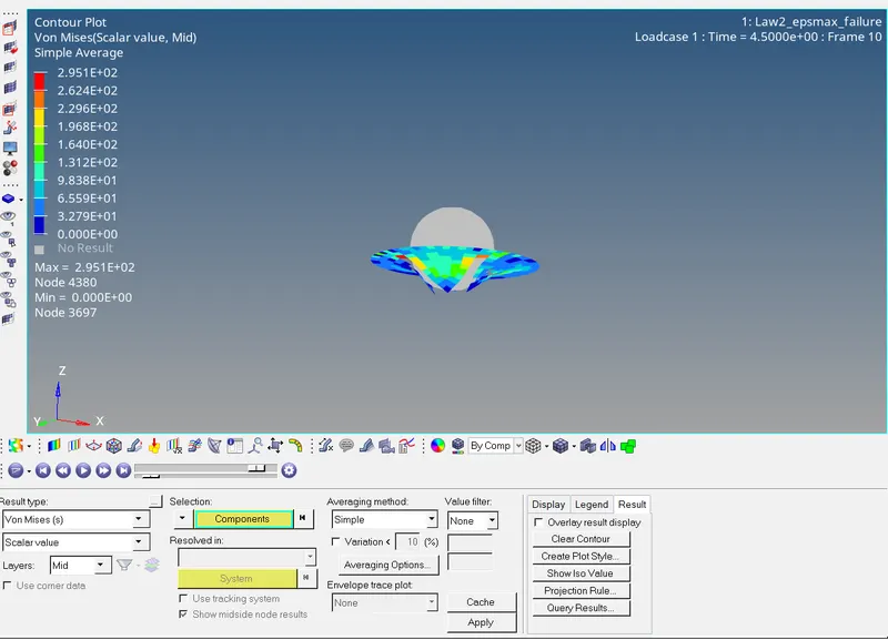
10.Check the energy and mass error.
11.The energy error is decent enough and is lesser than 5% and mass error is non existent.
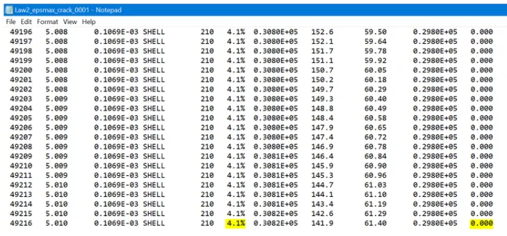
12.The highlighted potion are the end result.
GRAPHS:
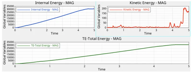
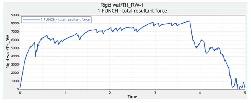
13.In this case, Ixfem is important here because it decides the way the elements react. With its value equal to 1 here it means the elements will crack and fail.
14.Along with Dadv crack propagation can also be seen here with elements being deleted only when the crack reaches them.
15.In this case, the rigid wall is moving. So to move any object there should be some external force is applying to the object.
16.That is why the rigid wall forces start increasing from zero and when it collided with the plate the energy got transferred to the elements thats the reason the rigid wall forces get decereased again to zero.
CASE-3:
1.Import the solver deck file Law2_epsmax_crack_0000.rad file.
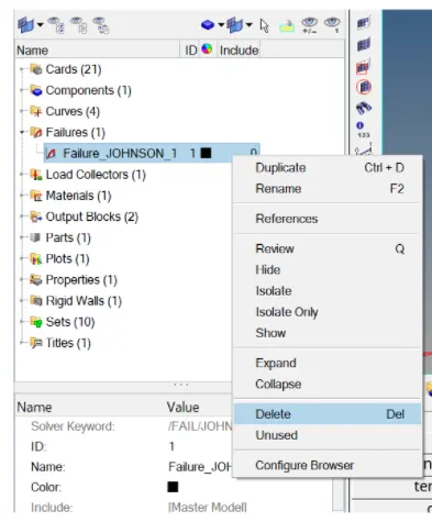
2.In this case delete the fail/JOHNSON card. Goto Failures > Failure_JOHNSON_1.
3.Run the analysis and save the file. With connectors ticked and -nt 4 typed in the option box we can click the RADIOSS button to run the analysis.
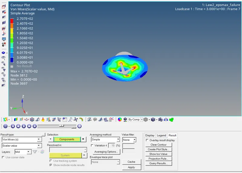
4.After the solver window completes the calculations, switch to HyperView window and run the h3hd file of the current analysis and set the Von Mises stress contours are attached in given section named as Case-3.
5.Check the energy and mass error on the RADIOSS output file Law2_epsmax_nofail_0001.out.
6.The energy error is almost 0 and the mass error is non existent. Now we switch to Hypergraph to plot the graphs.
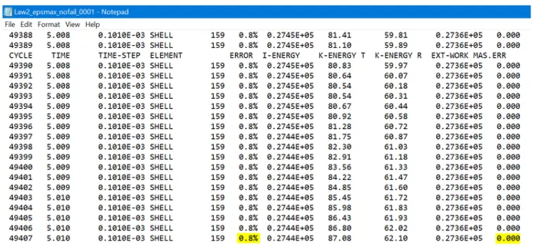
7.The highlighted potion are the end result.
GRAPHS:
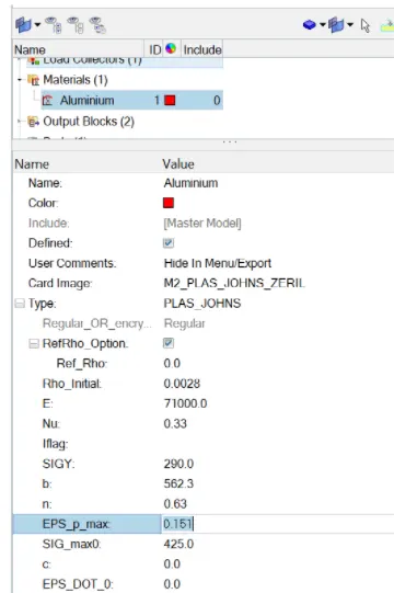
8.As we can see in the graph that its value is 0..151, meaning elements will be deleted if the strain on any integration point within said elements reaches 15.1% of the plastic strain.
9.The elements fail rapidly when compared to the elements is case-2 due to Xfem crack formulation there.
10.There is a linear increase in internal and total energy until a bulk of the elements are deleted from the model. This is expected since the energy absorbed by these elements go to waste due to their deletion.
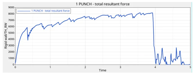
11.This is also explains the sudden drop in rigid wall forces at the same timestamp due to most elements that were in contact with the sphere during collision being deleted.
12.The rigid wall force is basically a measure of the opposing force generated by the metal sheet against the sphere.
13.Fluctuation occur when elements are deleted. When there are no elements to oppose the incoming sphere there wont be any rigid wall forces.
CASE-4:
1.Import the case-3 starter file Law2_epsmax_nofail_0001.rad.
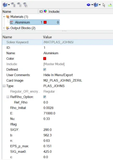
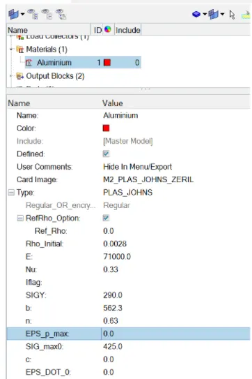
2.This time, delete the EPS_p_max value as 0. Going to the model tab we can go to Materials > Aluminium.
3.Now we can switch to the RADIOSS analysis section via Analysis > RADIOSS. Click on the connectors and type in -nt 4 in the options section and run the analysis by clicking RADIOSS.
4.After the solver finishes its analysis we can switch to Hyperview run Law2.h3hd, activate the Von Mises contours and the file is attached in the below section named case-4.
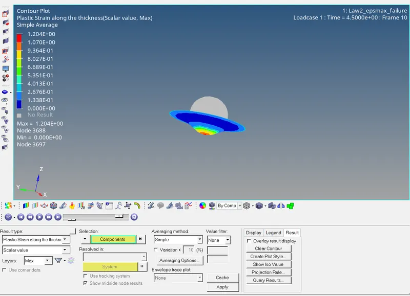
5.Now check the energy and mass errors on Law2_0001.out. The energy error is less than 5% and mass error is non-existent.
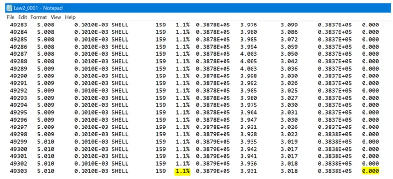
6.The highlighted potion are the end result.
GRAPHS:
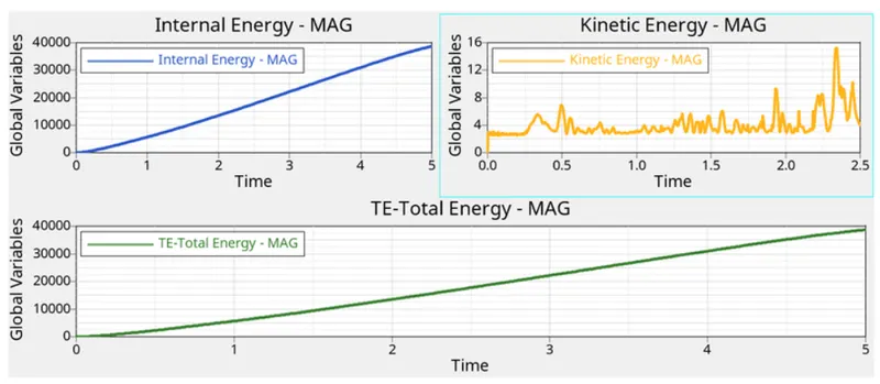
7.Law2 expresses material stress as a function of strain, strain rate and temperature.
8.The metal sheet is able to withstand a large amount of stress and avoid element deletion primarily due to the fact that the value for EPS_p_max was deleted.
9.RADIOSS assigns it the default value of 10^30. The fail/JOHNSON card was deleted. The material behaves like a pseudo-elastic material since it has a very high EPS_p_max threshold and elements cannot be deleted due to no failures cards.
10.With the value of c = 0, there is no strain rate. As a result the stress in this case is purely a function of strain generated in the material.
11.The kinetic energy generated in this case is almost negligible compared to the internal energy here. The total energy is increase is almost linear over time.
CASE-5:
1.Import the main starter file FAILURE_JOHNSON_0000.rad.
2.Goto Materials card > Aluminium and change the card image to M1_ELAST which is Law 1.
3.Set the values for Rho_Initial, E and Nu.
Rho_initial = 0.0028
E = 71000.00
nu= 0.33
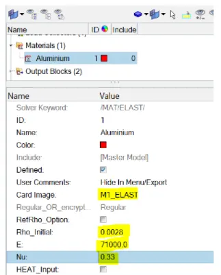
4.The highlighted portion is the changed conditions.
5.Do the analysis and save the file. Enable the connectors and type -nt 4 in the options box. Then we click RADIOSS and let the solver run the analysis.
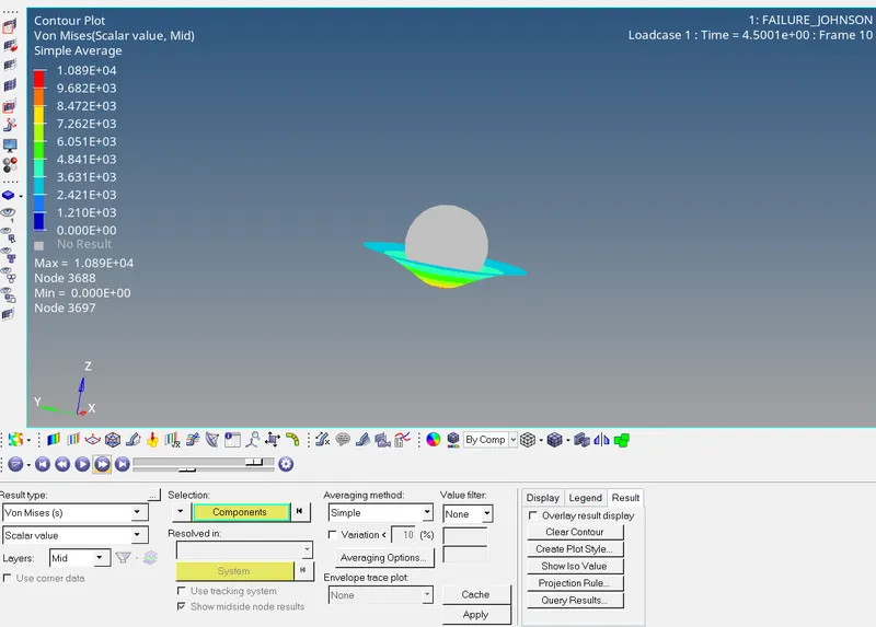
6.After the solver completes the analysis we switch to Hyperview, import the Law1.h3hd file, enable the Von Mises contours and the file is attached in below section named as Case-5.
6.Check the energy and mass error on the RADIOSS output file LAW1_0001.out.
7.The energy error is less than 5% and the mass error is non-existent. Now we switch to Hypergraph to plot the graphs for this simulations.
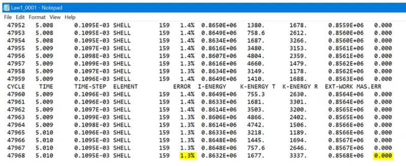
8.The highlighted potion are the end result.
GRAPHS:
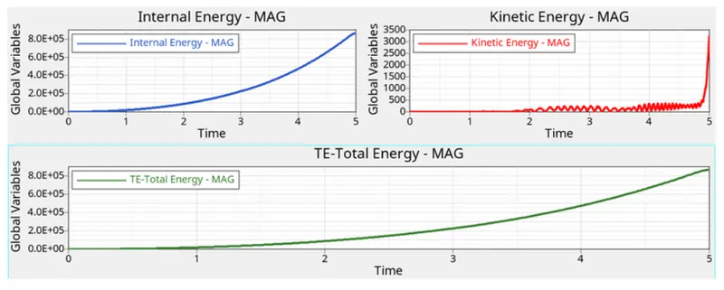
9.The plate is defined with a LAW-1 material which defines the basic properties of elastic material. This model considers only the elastic phase of the material, there is no plasticity involved which results in linear deformation.
10.In this case make use of the M1_Elast card. The metal sheet absorbs the full impact of the sphere.This material law is used to model purely elastic materials. This explains why there are no element deletions nor ruptures.
11.Due to its elasticity it also can absorb an extremely large amount of energy which explains the peak at the end of the kinetic energy plot. Absorbing a lot of energy also result in very high stresses-the maximum stress observed on the metal sheet is 10890 MPa, which is a massive value compared to the same in LAW2.
12.The kinetic energy gradually increases as the plate is stretched to the maximum limit for the applied load.
13.The internal energy keep increasing exponentially. The internal energy of the metal sheet increases due to the absorption of the kinetic energy from the impacting sphere and drops down once the plate returns to the original shape.
CASE-6:
1.Import the LAW27_0000.rad file.
2.We need to use recommended shell properties in this case. Goto Properties > 5NiP. Now we look at the utility window and set the following attributes.
I_shell = 24
I_smstr = 2
n = 2
N = 5
I_thick = 1
I_plas = 1
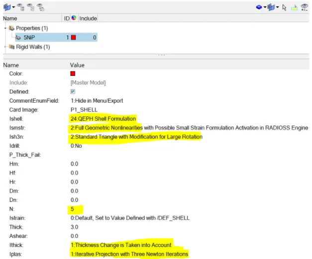
3.Run the analysis by the RADIOSS tool and save the file. We enable connectors and type -nt 4 in the options box. Then we click the RADIOSS and let the solver run the analysis.
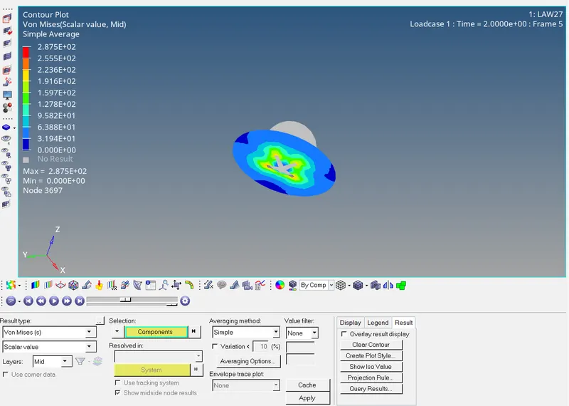
4.Now we can generate the simulation via Hyperview with the Von Mises contours and the file is attached in the below section named case-6.
5.Now we check the energy and mass error on Law_0001.out file.
6.The energy error is very close to 0 and the mass error is non existent.
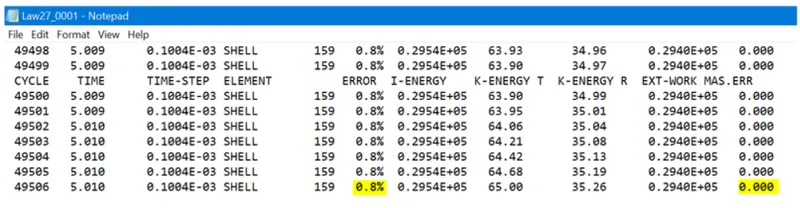
7.The highlighted potion are the end result.
GRAPHS:
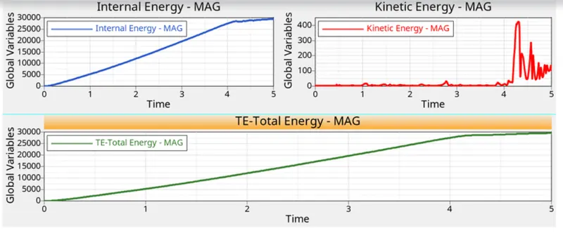
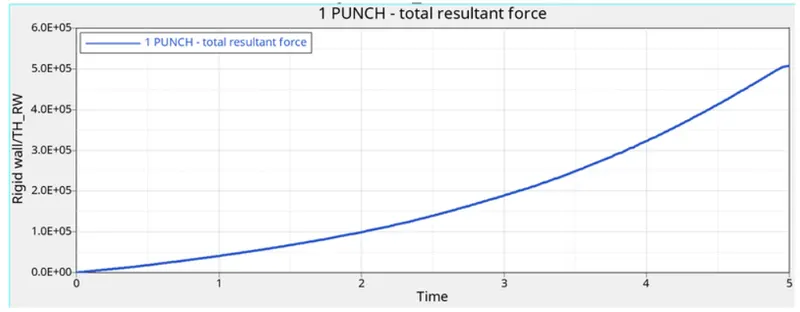
8.In this the use of the M27_PLAS_BRIT material card that is used for isotropic elastoplastic Johnson-Cook material model with an orthotropic brittle failure model.
9.The sheet absorbs more force and resorts to more deformation before the elements are deleted.
10.With the loss of energy through deleted elements, we notice the graph plateaus at around the 4ms mark.
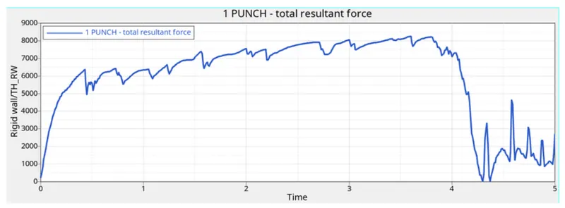
11.The several elements deleted and none to stop the incoming sphere, the rigid wall force graph drops at the same timestamp of 4m/s.
12.The spikes are formed when an element is deleted and is charcterized by a trough and crest but with so many elements deleted the trough is massive at 4ms mark.
CASE-7:
1.Import the LAW27_0000.rad file.
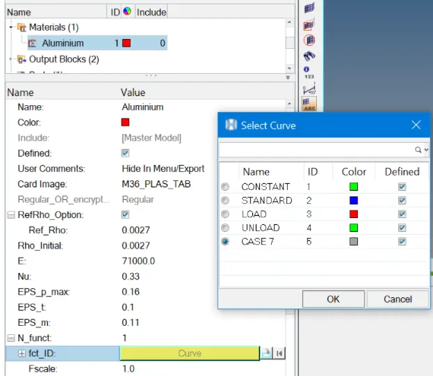
2.We will be editing certain attributes in this case. Go to model tab and we creating a new curve. Right click > Create > Curve.
3.Initially there are 4 curves we are adding the new curve named CASE 7.
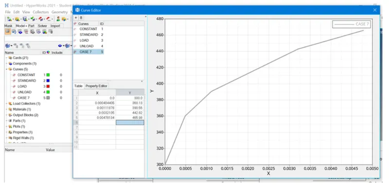
4.Goto Materials > Aluminium and change the card to M36_PLAS_TAB. After that set the values for Rho_Initial, E and Nu
Rho_Initial = 0.0027
E = 71000.00
nu = 0.33
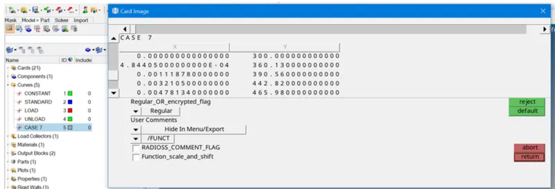
5.We can add the curve using the N_funct attribute. We can change its value to 1 and by doing so it lets us select the reference curve.
6.Now run the analysis using the Analysis > RADIOSS.
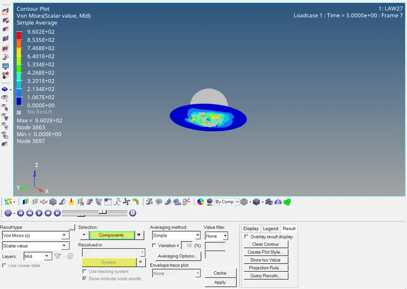
7.After the analysis is complete we switch to Hyperview and import the file with Von Mises Contours enabled and the file is attached in the given section named Case-7.
8.An energy error of -1.1% is acceptable since it is very close to 0.
9.The mass error is non-existent. Now we switch to Hypergraph to plot the graph.
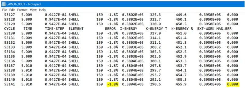
10.The highlighted potion are the end result.
GRAPHS:
11.From the simulation we can say that material exhibits strong brittle behaviour. It does not bend as much in response to the applied force and immediately disintegrates.
12.There seems to be not much cracking and the region of element deletion takes the shape of the sphere. We can notice is that the stress concentraion is localized around the region of impact and these stresses are not dissipated throughout the whole metal plate.
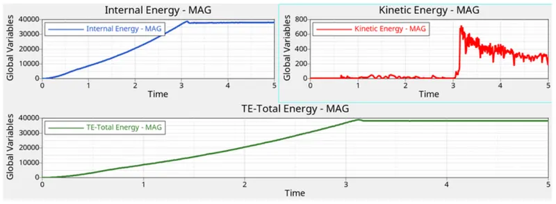
13.There is a linear relation between internal energy and time till past the 3 ms mark where many elements get deleted at once. When the elements are deleted the energy on each element goes to waste which results in the plateauing of curve.
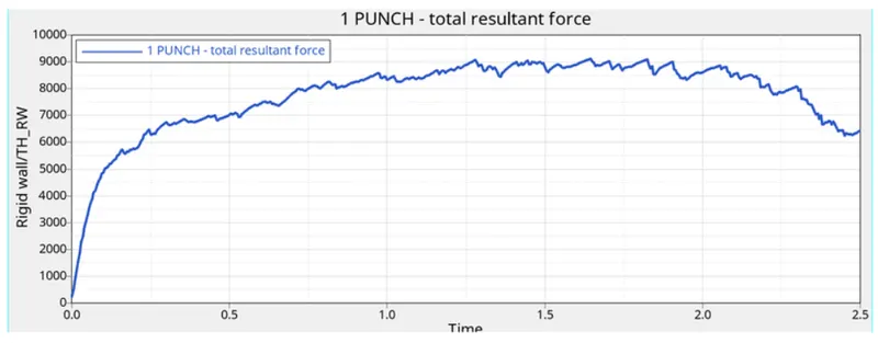
14.Each of the spikes is due to an element deletion. The resultant force gradually increases past the same 3ms mark which is when the sheet gives way and lets the sphere through.
15.With not much of sheet in the way, the rigid wall forces are drastically reduced and that results in that drop at the 3ms mark. The first drop occurs when the sheet reputures the first time.
Listed below is the comparision table for all the cases.
| Sl.No | Case | No.of cycles | Mass Error | Final Energy Error | Solver simulation time in seconds | Condition of elements under excessive stress |
| 1. | Case-1 | 49380 | 0 | 0.8% | 57.82 | Deleted |
| 2. | Case-2 | 49217 | 0 | 4.1% | 409.05 | Elements undergo crack formation and then deleted. |
| 3. | Case-3 | 49408 | 0 | 0.8% | 252.43 | Deleted |
| 4. | Case-4 | 48737 | 0 | 1.1% | 251.78 | Cannot be deleted due to lack of failure card and high default EPS_p_max value |
| 5. | Case-5 | 47969 | 0 | 1.3% | 194.29 | Cannot be deleted due to elastic card property |
| 6. | Case-6 | 49508 | 0 | 0.8% | 358.51 | Deleted |
| 7. | Case-7 | 53143 | 0 | -1.8% | 295.30 | Deleted |
OBSERVATION:
Selecting a correct material model plays a very important role in simulation. Selecting the wrong material model and doing simulation will also give result but it will not represent the actual situation.Thus for the
Law-1: It is used to model purely elastic materials.To model this we require Poisson's ratio and Young's modulus. This law represents a linear relationship between stress and strain.
Law-2: The material behaves as linear elastic when equivalent stress is lower than the yield stress. For a higher value of stress, the material behaves like plastic. Failure can be captured better with the help of an optional Fail_Johnson card.
Law-27: It is used for brittle materials.
Law-36: The elastic plastic behavior of isotropic material is modeled with user defined functions. The stress-strain curve is modeled using E and Poisson's ratio. Therefore it is best card because we cannot know the exact failing condition of the material in the other cases. But we can define the stress-strain curve and then we can decide where the material is failing.
RESULT:
Thus the simulation for the crash analysis on the given model by applying different materials laws is performed successfully and graphical output is obtained and comparision for all seven cases is worked sucessfully.