Assignment 4-RADIOSS Material Laws Challenge
Assignment 4: Radioss Materials Laws Challenge
Course: Crashworthiness Analysis using HyperMesh and Radioss
Submitted by: Amanpreet Singh Whan
Supervisor: Harsha Chowdary
December 26, 2021
List of Figures
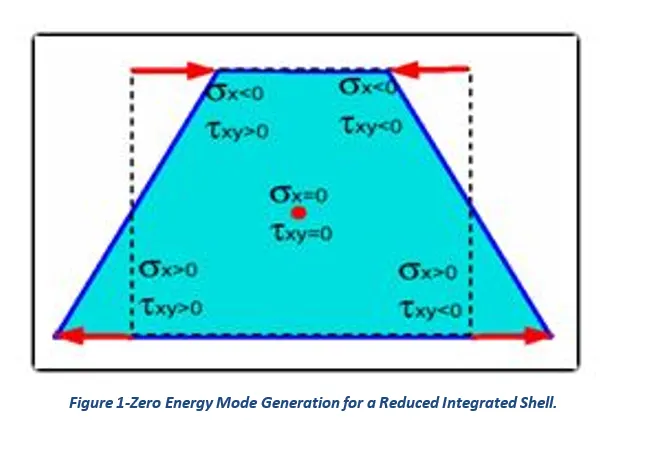
Figure 1-Zero Energy Mode Generation for a Reduced Integrated Shell.
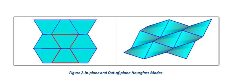
Figure 2-In-plane and Out-of-plane Hourglass Modes.
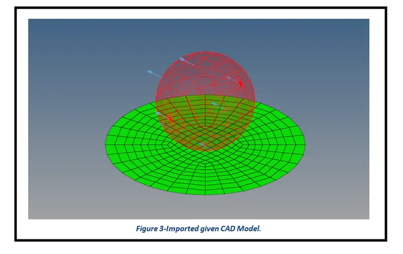
Figure 3-Imported given CAD Model.
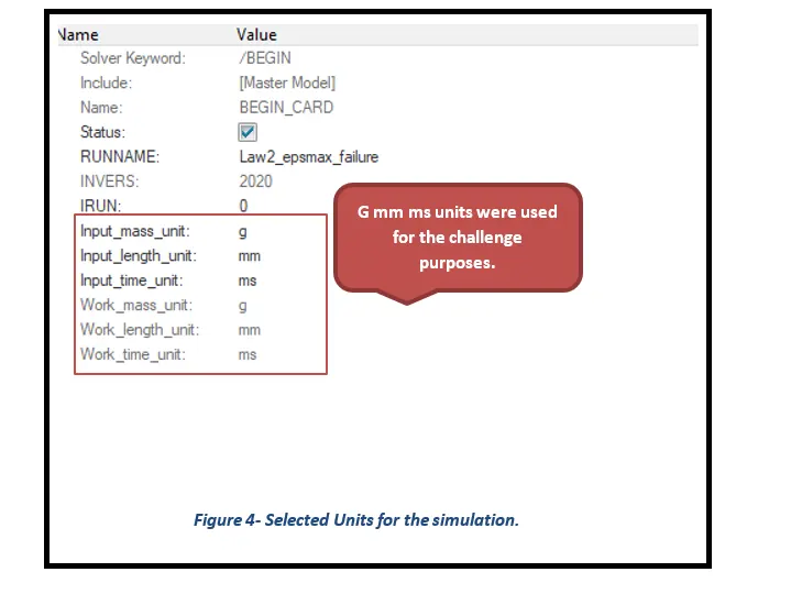
Figure 4- Selected Units for the simulation.
Figure 5- Material and Elemental properties used for Case 1.
Figure 6- The Procedure to be carried out to simulate in HyperMesh.
Figure 7-Rigid Wall Force results for the crash Case 1.
Figure 8-Global Energy plots for Case 1.
Figure 9-Energy and Mass error results for Case 1.
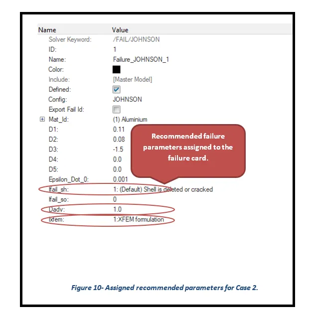
Figure 10- Assigned recommended parameters for Case 2.
Figure 11-Rigid Wall Force results for the crash Case 2.
Figure 12-Energy and Mass error results for Case 2.
Figure 13-Global Energy plots for Case 2.
Figure 14- Deletion of Failure card for Case 3.
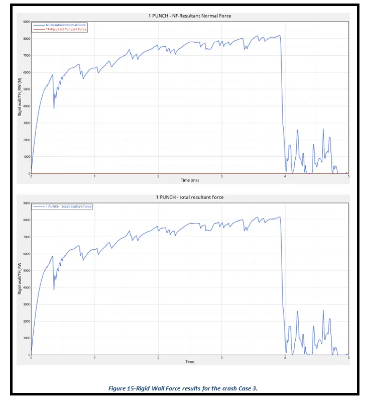
Figure 15-Rigid Wall Force results for the crash Case 3.
Figure 16- Energy and Mass error results for Case 3.
Figure 17-Global Energy plots for Case 3.
Figure 18- Deletion of Eps_p_max value for Case 4.
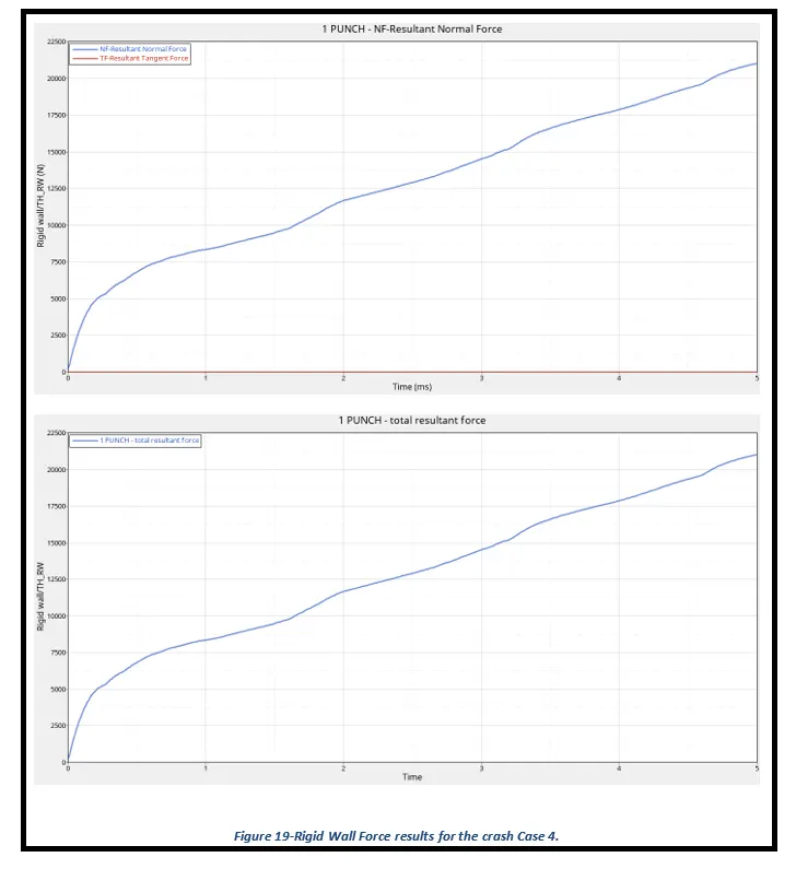
Figure 19-Rigid Wall Force results for the crash Case 4.
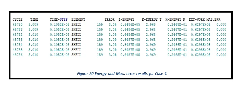
Figure 20-Energy and Mass error results for Case 4.
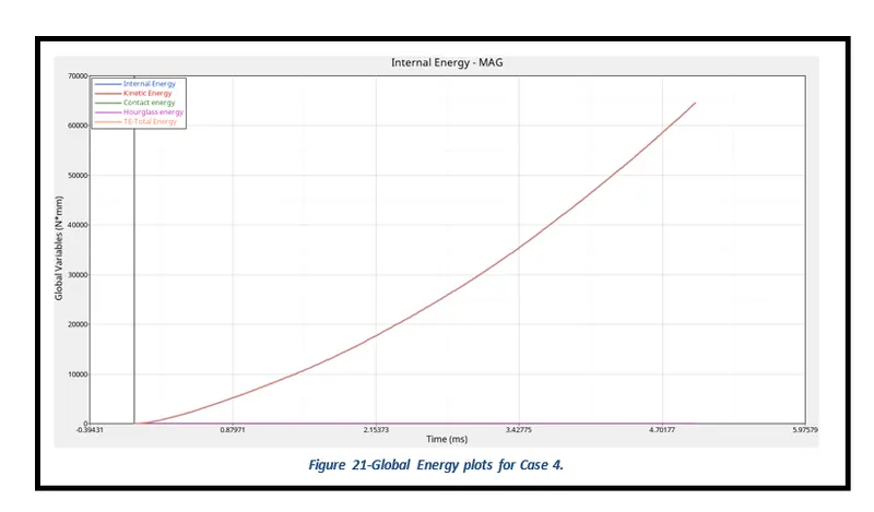
Figure 21-Global Energy plots for Case 4.
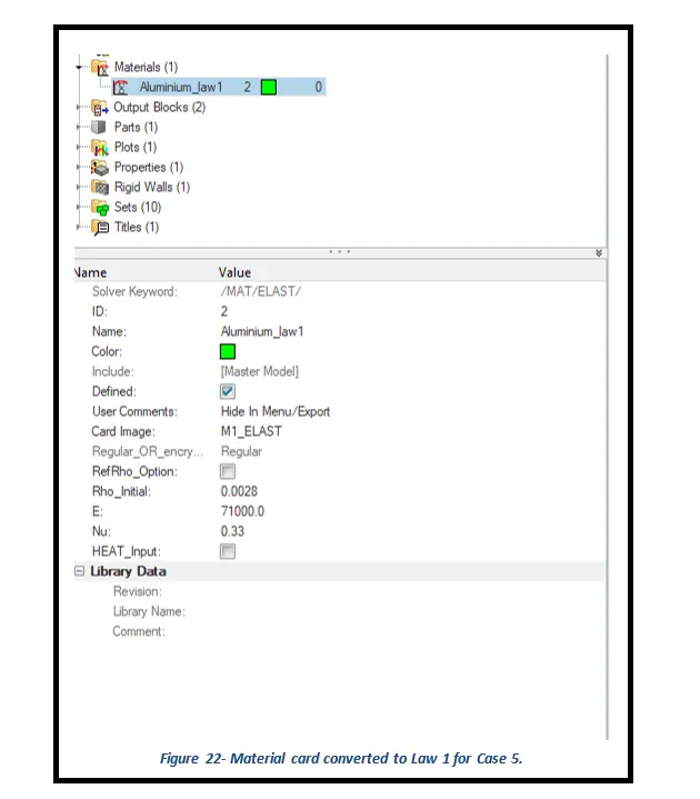
Figure 22- Material card converted to Law 1 for Case 5.
Figure 23-Rigid Wall Force results for the crash Case 5.
Figure 24-Energy and Mass error results for Case 5.
Figure 25-Global Energy plots for Case 5.
Figure 26-Rigid Wall Force results for the crash Case 6.
Figure 27-Energy and Mass error results for Case 6.
Figure 28-Global Energy plots for Case 6.
Figure 29- Material card created using Law 36 for Case 7.
Figure 30-Rigid Wall Force results for the crash Case 7.
Figure 32-Energy and Mass error results for Case 7.
Figure 31-Global Energy plots for Case 7.
Table of Contents
3.2 Creating Input Deck for running simulation.
1 Introduction
HyperMesh is the market-leading, multi-disciplinary finite element pre-processor which manages the generation of the largest, most complex models, starting with the import of CAD geometry to exporting a ready-to-run solver file. HyperMesh supports a wide variety of CAD and solver interfaces, making it a perfect solution for most industry verticals and domains. With its advanced geometry and meshing capabilities, HyperMesh provides an environment for rapid model generation. Generating high-quality mesh quickly is just one of Hyper Mesh’s core competencies. For complex sub-system generation and assembly, HyperMesh has advanced model assembly tools. Modeling of laminate composites is supported by advanced creation, editing, and visualization tools. Design changes can be made easily via mesh morphing and geometry dimensioning.
Theory
Element Configurations: Each element has an associated element configuration. An element configuration tells HyperWorks how to draw, store, and work with the element.
- 1D Elements include Spring, Trusses, and Beam elements.
- 2D Elements include Quads and Trias.
- 3D Elements include Solid Elements such as Hexa and Tetra elements.
Hourglass Formulations: Hourglass (HG) modes are nonphysical, zero-energy modes of deformation that produce zero strain and no stress. Hourglass modes occur only in under-integrated (single integration point) solid, shell, and thick shell elements.
As shown in Figure 2 for an anti-symmetric deformation of a shell element with one integration point at the center, a zero-energy mode can be found for a physical deformation mode. That cannot be true from a physical point of view and must be corrected. For a shell mesh, the two main hourglass modes are in-plane (membrane mode) and out-of-plane (W mode).
The two correcting methods available are:
- Perturbation or penalty method: Hourglass control by application of anti-hourglass forces to maintain deformation stability of the element.
- Physical stabilization method: Hourglass control by the correction of internal energy in an analytical way.
For the first method, four formulations are available in Radioss:
- Type 1 (Default option): Only in-plane modes are corrected, valid for shells and solids.
- Type 2: Old formulation no longer recommended.
- Type 3: Plasticity is considered in the computation of anti-hourglass forces; in-plane and out-of-plane hourglass modes are corrected; available only for shells.
- Type 4: Like Type 1 with additional higher-order terms in the computation of anti-hourglass forces and with out-of-plane hourglass mode correction; available only for shells.
The second method is powerful and can be used when the mesh quality is good. The physical stabilization method is incorporated in the following Radioss elements:
- QEPH shell
- HEPH solid
- HSEPH solid shell
The choice of hourglass formulation plays an essential role in the quality of results. If the mesh is fine enough, the physical stabilization method can be used. Otherwise, Type 3 and Type 4 formulations are recommended for shell meshes. When the material undergoes elastic-plastic behavior, the Type 3 formulation is much more efficient. The hourglass coefficient, hm and hf are recommended to be set to 0.1; however, the default value, hf=0.01 can be used for hr.
Best Element Formulation for the Crash Analysis:
|
Parameters |
Comment |
|
Ishell = 24 |
QEPH 4 nodes shells are the best combination of cost and accuracy |
|
Ismstr = 2 |
Full geometric nonlinearities with possible small strain formulation activation in RADIOSS Engine. |
|
Ish3n= 2 |
Standard 3 noded shell (C0) with modification for large rotation |
|
N = 5 |
The number of integration points is set to 5 for accuracy bending. |
|
Ithick = 1 |
Thickness change is considered for accuracy. |
|
Iplas = 1 |
Iterative plasticity for good accuracy. |
Material Laws:
A large variety of materials is used in the structural components and must be modeled in stress analysis problems. For any kind of these material, a range of constitutive laws is available to describe by a mathematical approach the behavior of the material.
The choice of a constitutive law for a given material depends at first on the desired quality of the model. For example, for standard steel, the constitutive law may take into account the plasticity, anisotropic hardening, strain rate, and temperature dependence. However, for a routine design may be a simple linear elastic law without strain rate and temperature dependence is sufficient to obtain the needed quality of the model.
Radioss material library contains several distinct material laws. The constitutive laws may be used by the analyst for general applications or a particular type of analysis. The available materials are categorized into the following groups:
- Elasto-plasticity Materials
- Hyper and Visco-elastic Materials
- Composite and Fabric
- Concrete and Rock
- Honeycomb
- Multi-Material, Fluid, and Explosive Materials
- Other Materials (contain fictitious, porous, gas materials, etc.)
Isotropic Elastic Material
Two kinds of isotropic elastic materials are considered:
- Linear elastic materials with Hooke’s law,
- Nonlinear elastic materials with Ogden, Mooney-Rivlin, and Arruda-Boyce laws.
Linear Elastic Material (LAW 1): This material law is used to model purely elastic materials or materials that remain in the elastic range. Hooke's law requires only two values to be defined: the Young's or elastic modulus E and Poisson’s Ratio ν. The law represents a linear relationship between stress and strain.
Ogden Materials (LAW 42, LAW 69, and LAW 82): Ogden's law is applied to slightly compressible materials like rubber or elastomer foams undergoing large deformation with an elastic behavior.
Ogden Material LAW 69: This law similar to MAT LAW 42 (OGDEN) defines a hyperelastic and incompressible material specified using the Ogden or Mooney-Rivlin material models. Unlike LAW 42 where the material parameters are input, this law computes the material parameters from an input engineering stress-strain curve from uniaxial tension and compression tests. This material can be used with shell and solid elements.
Yeoh Material LAW 94: The Yeoh model is a hyperelastic material model that can be used to describe incompressible materials. The strain energy density function of LAW 94 only depends on the first strain invariant.
Composite and Anisotropic Materials
The orthotropic materials can be classified into the following cases:
- Linear elastic orthotropic shells as fabric
- Nonlinear orthotropic pseudo-plastic solids as honeycomb materials
- Elastic-plastic orthotropic shells
- Elastic-plastic orthotropic composites
Fabric Law for Elastic Orthotropic Shells LAW 19 and LAW 58:-
Fabric Linear Law for Elastic Orthotropic Shells LAW19: A material is orthotropic if its behavior is symmetrical with respect to two orthogonal planes. The fabric law enables to the model of this kind of behavior. This law is only available for shell elements and can be used to model an airbag fabric. Many of the concepts for this law are the same as for LAW14 which is appropriate for composite solids.
Fabric Nonlinear Law for Elastic Anisotropic Shells LAW 58: This law is used with Radioss standard shell elements and anisotropic layered property (TYPE16). The fiber directions (warp and weft) define the local axes of anisotropy. Material characteristics are determined independently in these axes.
Conventional Nonlinear Pseudo-Plastic Orthotropic Solids LAW28 and LAW 50: These laws are generally used to model honeycomb material structures as crushable foams. The microscopic behavior of this kind of material can be considered as a system of three independent orthogonal springs. The nonlinear behavior in orthogonal directions can then be determined by experimental tests. The behavior curves are injected directly into the definition of law. Therefore, the physical behavior of the material can be obtained by a simple law. However, the microscopic elastoplastic behavior of a material point cannot be represented by decoupled unidirectional curves. This is the major drawback of the constitutive laws based on this approach. The cell direction is defined for each element by a local frame in the orthotropic solid property.
Hill's Law for Orthotropic Plastic Shells: Hill's law models an anisotropic yield behavior. It can be considered as a generalization of von Mises yield criteria for anisotropic yield behavior.
Elastic-plastic Orthotropic Composite Shells LAW 15 and LAW 25: Two kinds of composite shells may be considered in the modeling:
- Composite shells with isotropic layers
- Composite shells with at least one orthotropic layer
The first case can be modeled by an isotropic material where the composite property is defined in the element property definition. However, in the case of the composite shells with orthotropic layers, the definition of a convenient material law is needed. Two dedicated material laws for composite orthotropic shells exist in Radioss:
- Material law COMPSH (25) with orthotropic elasticity, two plasticity models, and brittle tensile failure,
- Material law CHANG (15) with orthotropic elasticity, fully coupled plasticity, and failure models.
Elastic-Plastic Orthotropic Composite Solids LAW 14: The material LAW14 (COMPSO) in Radioss allows to simulate orthotropic elasticity, Tsai-Wu plasticity with damage, brittle rupture, and strain rate effects. The constitutive law applies to only one layer of the lamina. Therefore, each layer needs to be modeled by a solid mesh. A layer is characterized by one direction of the fiber or material. The overall behavior is assumed to be elastoplastic orthotropic.
Elastic-plasticity of Isotropic Materials
The strain hardening behavior of materials is a major factor in structural response as metalworking processes or plastic instability problems. A proper description of strain hardening at large plastic strains is generally imperative. For many plasticity problems, the hardening behavior of the material is simply characterized by the strain-stress curve of the material. For the proportional loading, this is generally true. However, if the loading path is combined, the characterization by a simple strain-stress curve is no longer adequate.
The incremental plasticity theory is generally used in computational methods. Plasticity models are written as rate-dependent or independent. A rate-dependent model is one in which the strain rate does affect the constitutive law. This is true for a large range of metals at low temperatures relative to their melting temperature. Most isotropic elastic-plastic material laws in Radioss use von Mises yield criteria as given in stresses in solids.
Johnson-Cook Plasticity Model LAW 2: In this law, the material behaves as linear elastic when the equivalent stress is lower than the yield stress.
Zerilli-Armstrong Plasticity Model LAW2: This law is similar to the Johnson-Cook plasticity model. The same parameters are used to define the work hardening curve.
Cowper-Symonds Plasticity Model LAW 44: This law models an elastoplastic material with:
- Isotropic and kinematic hardening
- Tensile rupture criteria
The damage is neglected in the model. The work hardening model is similar to the Johnson-Cook model (LAW2) without temperature effect where the only difference is in the strain rate dependent formulation.
Tabulated Piecewise Linear and Quadratic Elasto-plastic Laws LAW 36 and LAW 60: The elastic-plastic behavior of isotropic material is modeled with user-defined functions for work hardening curve. The elastic portion of the material stress-strain curve is modeled using the elastic modulus E, and Poisson's ratio υ. The hardening behavior of the material is defined in the function of plastic strain for a given strain rate. An arbitrary number of material plasticity curves can be defined for different strain rates. For a given strain rate, a linear interpolation of stress for plastic strain change can be used. This is the case of LAW 36 in Radioss. However, in LAW 60 a quadratic interpolation of the functions allows to better simulate the strain rate effects on the behavior of the material as it is developed in LAW 60.
Drücker-Prager LAW 10, LAW 21, and LAW 81: For materials, like soils and rocks, the frictional and dilatational effects are significant. In these materials, the plastic behavior depends on the pressure as the internal friction is proportional to the normal force.
Brittle Damage Johnson-Cook Plasticity Model LAW 27: Johnson-Cook plasticity model is presented in Johnson-Cook Plasticity Model (LAW2). For shell applications, a simple damage model can be associated with this law to take into account the brittle failure. The crack propagation occurs in the plan of shell in the case of mono-layer property and through the thickness if a multi-layer property is defined.
Brittle Damage Reinforced Concrete Material LAW 24: The model is a continuum, plasticity-based, damage model for concrete. It assumes that the main two failure mechanisms are tensile cracking and compressive crushing of the concrete material. The material law will enable to the formulation of the brittle elastic-plastic behavior of the reinforced concrete.
Ductile Damage Model for Porous Materials LAW 52: The Gurson constitutive law models progressive micro rupture through void nucleation and growth. It is dedicated to high strain rate elasto-viscoplastic porous metals. A coupled damage mechanical model for strain rate-dependent voided material is used.
2 Aims
- Run a total of seven different crash simulations using different material card laws or properties as per the challenge requirements.
- Perform mass and energy checks and determine whether the results are acceptable or not.
- Plot and tabulate the total number of cycles, Simulation Time, Rigid Wall Forces, Internal Energy, Hourglass Energy, Contact Energy, Total Energy results for the performed simulations and compare the results for the same.
3 Methodology and Results
The section describes the different stages that were performed using an engineering tool HyperWorks Radioss 2020 for the completion of the Assignment 4 Challenge. These stages can be further broadly sub-categorized into three key steps, starting from importing of cad model to creating simulation cards and finally performing the crash simulation to obtain desired results.
3.1 Importing of CAD Model
After opening the HyperWorks software, the first step is to select the Radioss profile and then open the given CAD model.
3.2 Creating Input Deck for running simulation
In HyperMesh (Radioss), there are certain key cards that have to be defined in order to run a successful simulation and also to obtain the desired results. A total of seven different crash tests with different material laws or properties were performed to fulfill the requirements of the given challenge. The simulations run for the given rupture plate CAD model are of the following order.
- Case 1: Law2_epsmax_failure
- Case 2: Law2_epsmax_crack
- Case 3: Law2_epsmax_nofail
- Case 4: Law 2 Johnson Cook plastic
- Case 5: Law 1 Elastic
- Case 6: Law 27 Plas Brittle
- Case 7: Law 36 Elasto Plastic
What follows hereafter is the images representing the given Input Deck along with the obtained results from the simulations performed for the different seven cases.
Case 1: Law 2_epsmax_failure
After importing the given Rupture Plate CAD Model in the HyperMesh, the first and foremost step is to set up the analysis units, g mm ms was chosen to be the most appropriate units for this challenge. The following figure illustrates the units selected for the crash test of the given model.
The challenge requirement for Case 1 was to run the simulation without making any changes in the material and element properties of the given model. Thus, the values used for the material properties and elemental formulations are presented in the following figures.
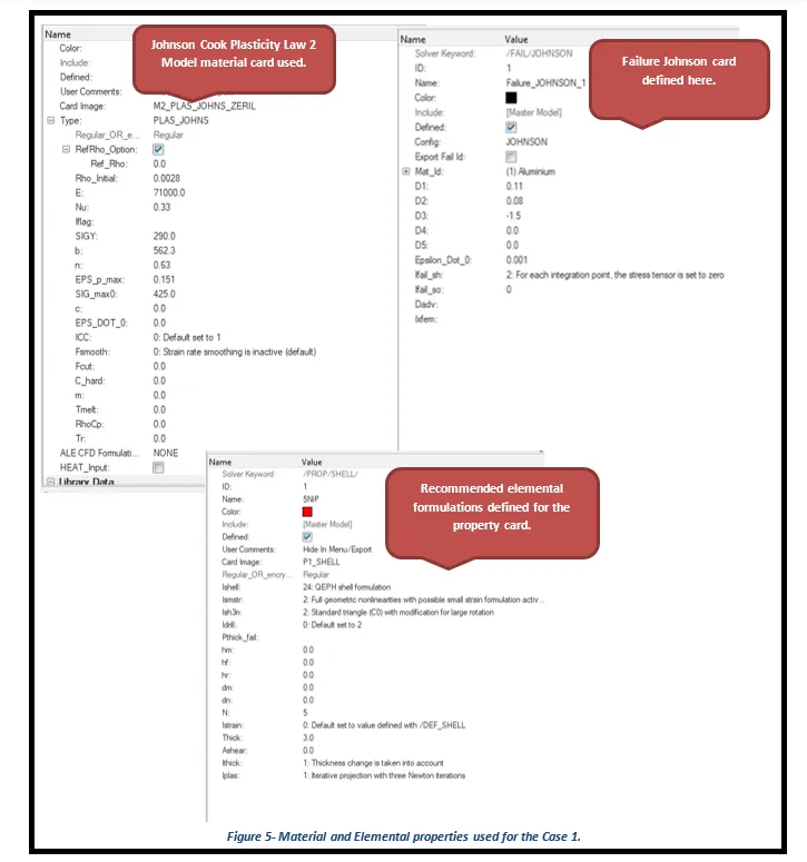
The crash simulation can be performed using the following process.
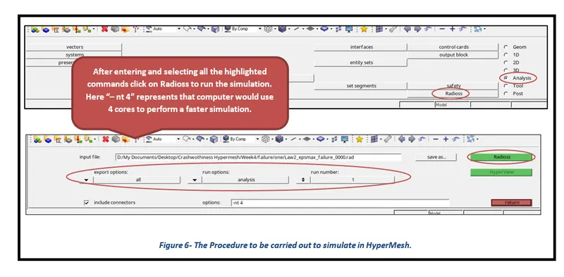
- Go to Analysis Deck -> Select Radioss -> Change Input file to Law2_epsmax_failure_0000 -> Select all for Export options -> Analysis for Run Options -> Select 1 for the Run number -> Tick include connectors -> Enter “-nt 4” for the options -> Hit Radioss to run simulation.
Case 1- Law 2_epsmax_failure Simulation Results
To visualize the simulation, either split the graphic interface into two to open the Hyper View utility or open the Hyper View window from the Post toolbar. Import the “h3d” file generated by the Radioss from the saved directory and then visualize the desired results using relevant commands. To plot rigid wall forces or other global forces, open the HyperGraph 2D interface and import the “T01” file, and plot the desired graphs.
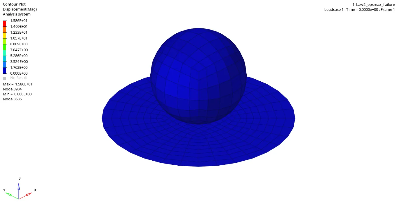
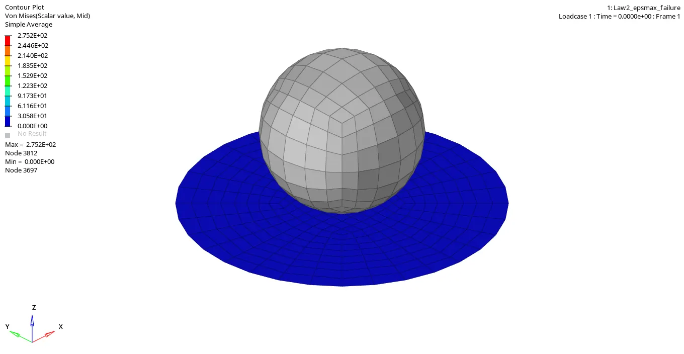
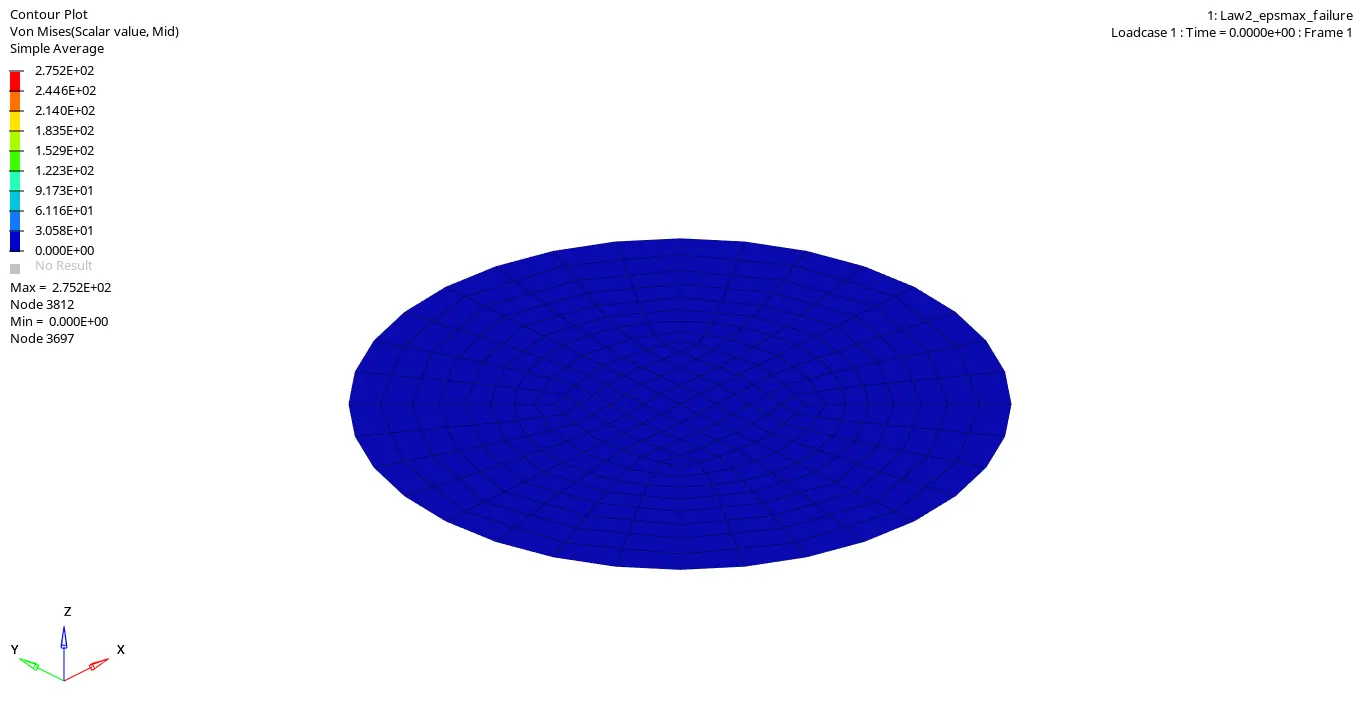
From the simulation results, it was observed that the maximum displacement experienced by the plat elements before getting deleted was around 15.86 mm while the maximum stress generated on the plate was around 275.2 MPa.
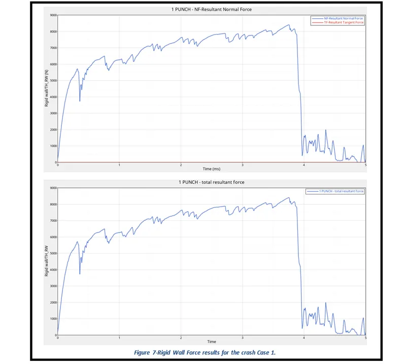
The rigid wall forces are generally the forces experienced by the wall during a crash test. For the challenge purposes, the Total Resultant Force graphs were plotted for both the crash test analysis. From Figure 7, it can be seen that the Net Resultant Normal force of the rigid wall is exactly identical to the Net Resultant Force of the rigid wall. It can also be seen that the Net Resultant force continuously increases between 0 to 3.97 ms and then it drops significantly and becomes 0 at the end of the simulation. The drops in the magnitude of resultant forces have essentially occurred due to the deletion of the elements.
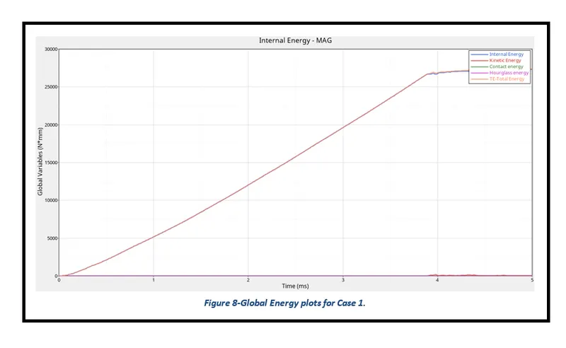
The Total Energy reported by Global variables in Radioss is the sum of internal energy, kinetic energy, contact (sliding) energy, hourglass energy system, damping energy, and rigid wall energy. What can be interpreted from Figure 8 is that the circular plate resists the motion of the rigid sphere until 3.9 ms and after that, the plate gets ruptured completely by it. Thus, proving that both the kinetic and internal energy increases up to the value of 27000 N*mm and as soon as the plate allows the sphere to pass through, both the energies become constant.
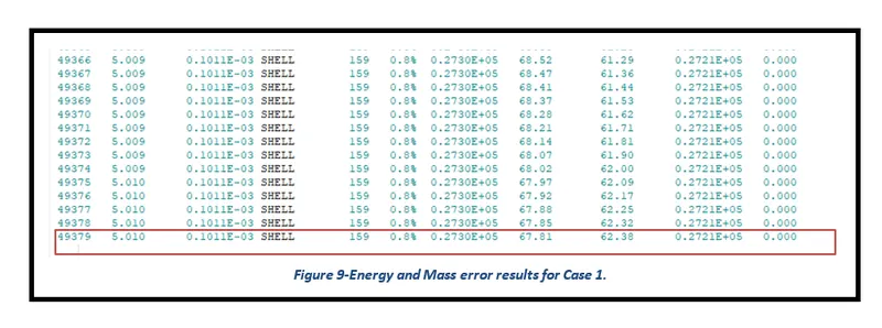
The Energy error should be negative and decrease with the iterations. Thus, ideally, the error should be at most -15% and better to have 5%. The closer to 0% error the better. The Mass error of less than 2% is preferred for the crash simulations. From Figure 9, it can be noted that the simulation yields an Energy Error of 0.8% which is close to 0 and therefore acceptable. However, the Mass error generated by the simulation for case 1 is 0%.
Case 2: Law 2_epsmax_Crack
The simulation for Case 2 is performed using the same process that was carried out for Case 1. However, the Failure Johnson card parameters were assigned the following values.
- Ifail_sh = 1 ; Dadv = 1 ; Ixfem = 1
Case 2- Law 2_epsmax_crack Simulation Results
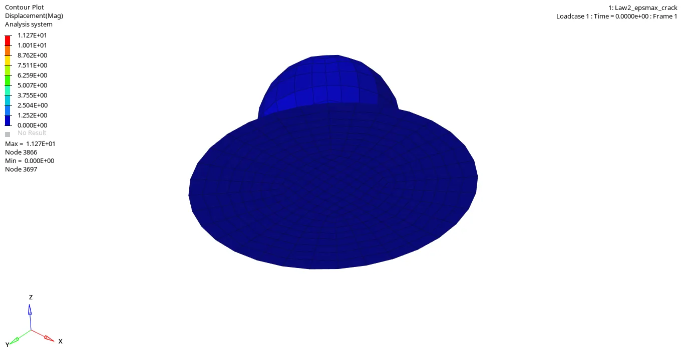
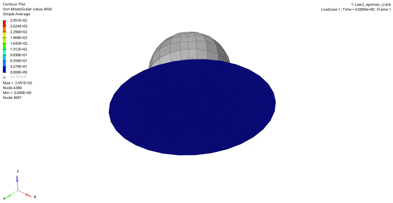
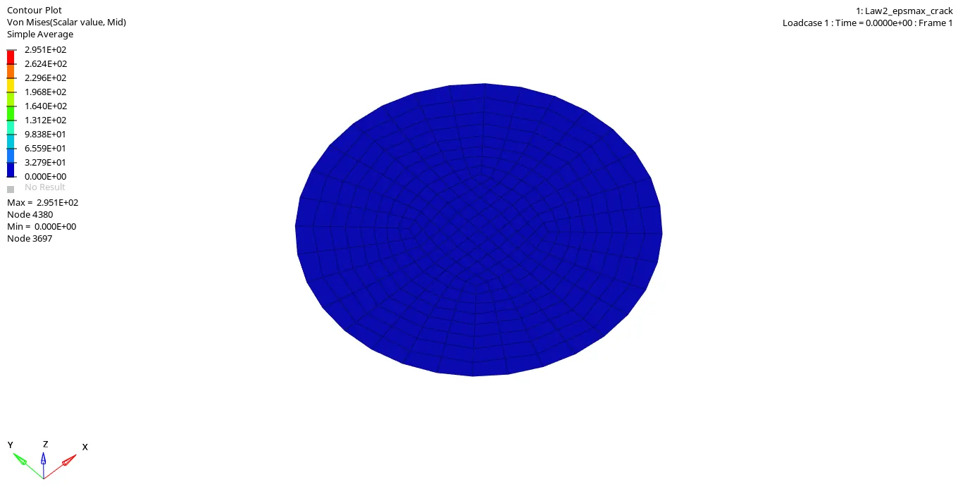
From the simulation results, it was observed that the maximum displacement experienced by the plat elements before getting deleted was around 11.27 mm while the maximum stress generated on the plate was around 295.1 MPa.
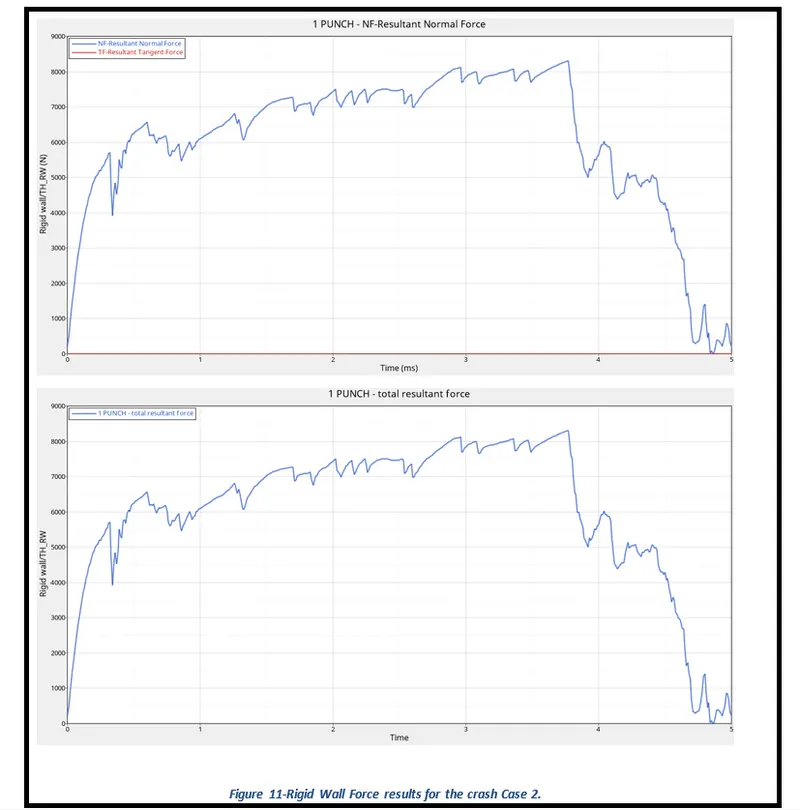
The rigid wall forces are generally the forces experienced by the wall during a crash test. For the challenge purposes, the Total Resultant Force graphs were plotted for both the crash test analysis. From Figure 11, it can be seen that the Net Resultant Normal force of the rigid wall is exactly identical to the Net Resultant Force of the rigid wall. It can also be seen that the Net Resultant force continuously increases between 0 to 4.7 ms and then it drops significantly and varies a bit and becomes 0 at the end of the simulation. The drops in the magnitude of resultant forces have essentially occurred due to the development of cracks and the deletion of the elements.
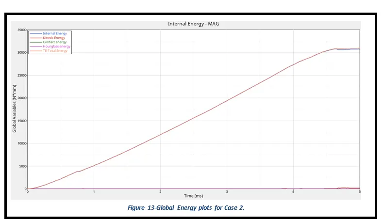
The Total Energy reported by Global variables in Radioss is the sum of internal energy, kinetic energy, contact (sliding) energy, hourglass energy system, damping energy, and rigid wall energy. What can be interpreted from the Figure 13 is that the circular plate resists the motion of the rigid sphere until 4.7 ms and after that, the plate gets ruptured completely by it. Thus, proving that both the kinetic and internal energy increases up to the value of 30650 N*mm and as soon as the plate allows the sphere to pass through both the energies become constant.
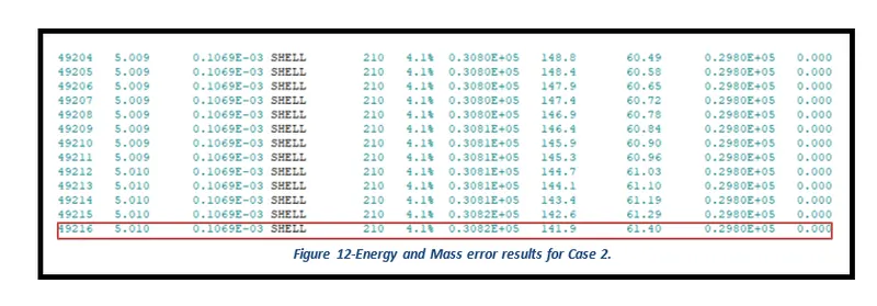
The Energy error should be negative and decrease with the iterations. Thus, ideally, the error should be at most -15% and better to have 5%. The closer to 0% error the better. The Mass error of less than 2% is preferred for the crash simulations. From Figure 12, it can be noted that the simulation yields an Energy Error of 4.1% while the Mass error generated by the simulation for this case is 0%.
Case 3 : Law 2_epsmax_no fail
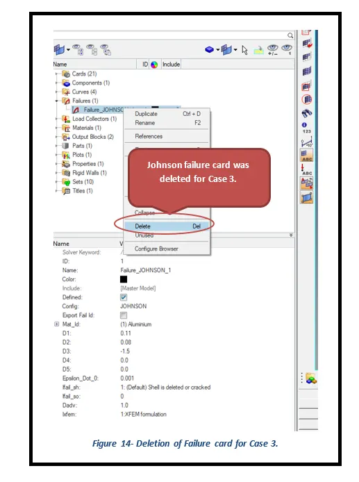
The simulation for Case 3 is performed using the same process that was carried out for Case 2. However, the Failure Johnson card was deleted for this case.
Case 3- Law 2_epsmax_no fail Simulation Results
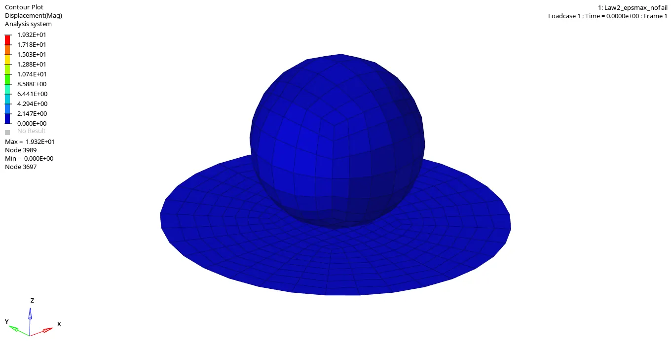
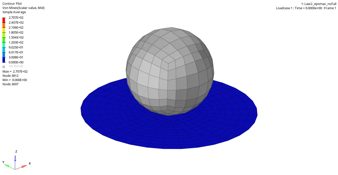
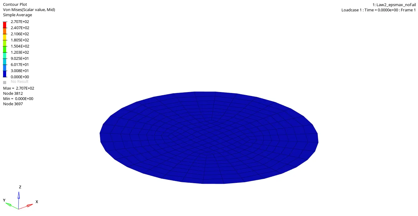
From the simulation results, it was observed that the maximum displacement experienced by the plat elements before getting deleted was around 19.32 mm while the maximum stress generated on the plate was around 270.7 MPa.
The rigid wall forces are generally the forces experienced by the wall during a crash test. For the challenge purposes, the Total Resultant Force graphs were plotted for both the crash test analysis. From Figure 15, it can be seen that the Net Resultant Normal force of the rigid wall is exactly identical to the Net Resultant Force of the rigid wall. It can also be seen that the Net Resultant force continuously increases between 0 to 3.9 ms and then it drops significantly and varies a bit and becomes 0 at the end of the simulation. The drops in the magnitude of resultant forces have essentially occurred due to the deletion of the elements.
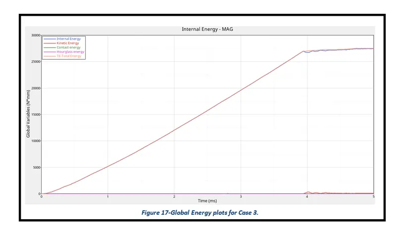
The Total Energy reported by Global variables in Radioss is the sum of internal energy, kinetic energy, contact (sliding) energy, hourglass energy system, damping energy, and rigid wall energy. What can be interpreted from the Figure 17 is that the circular plate resists the motion of the rigid sphere until 4.7 ms and after that, the plate gets ruptured completely by it. Thus, proving that both the kinetic and internal energy increases up to the value of 30650 N*mm and as soon as the plate allows the sphere to pass through both the energies become constant.
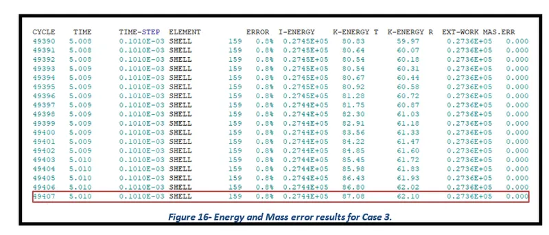
The Energy error should be negative and decrease with the iterations. Thus, ideally, the error should be at most -15% and better to have 5%. The closer to 0% error the better. The Mass error of less than 2% is preferred for the crash simulations. From Figure 16, it can be noted that the simulation yields an Energy Error of 0.8% while the Mass error generated by the simulation for this case is 0%.
Case 4: Law 2 Johnson Cook Plastic
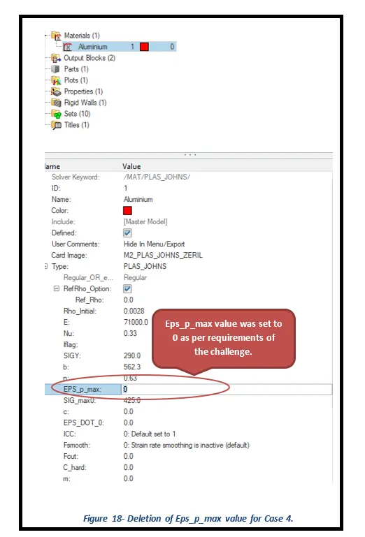
The simulation for Case 4 is performed using the same process and the same starter file that was used for Case 3. However, the Eps_p_max value was deleted for this case.
Case 4- Law 2 Simulation Results
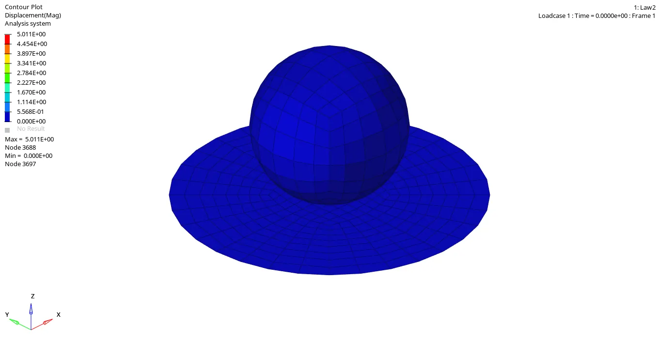
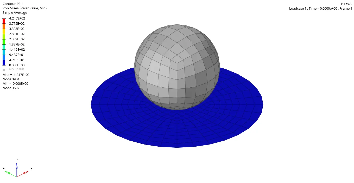
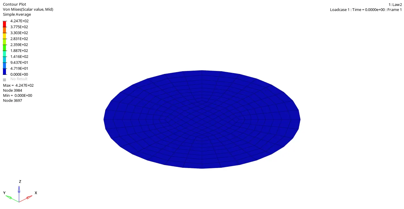
From the simulation results, it was observed that the maximum displacement experienced by the plat elements before getting deleted was around 5.01 mm while the maximum stress generated on the plate was around 424.7 MPa.
The rigid wall forces are generally the forces experienced by the wall during a crash test. For the challenge purposes, the Total Resultant Force graphs were plotted for both the crash test analysis. From Figure 19, it can be seen that the Net Resultant Normal force of the rigid wall is exactly identical to the Net Resultant Force of the rigid wall. It can also be seen that the Net Resultant force and Resultant Normal force both increase constantly throughout the simulation. This has essentially occurred because of the absence of failure criterion in the Material card.
The Total Energy reported by Global variables in Radioss is the sum of internal energy, kinetic energy, contact (sliding) energy, hourglass energy system, damping energy, and rigid wall energy. What can be interpreted from the Figure 21 is that the Kinetic Energy, Internal Energy, and Total Energy of the system increase constantly as there is an absence of the failure criterion in the material card. In addition, it can be observed that the Contact and Hourglass Energy remains constant and negligible.
The Energy error should be negative and decrease with the iterations. Thus, ideally, the error should be at most -15% and better to have 5%. The closer to 0% error the better. The Mass error of less than 2% is preferred for the crash simulations. From Figure 20, it can be noted that the simulation yields an Energy Error of 3% while the Mass error generated by the simulation for this case is 0%.
Case 5: Law 1 Elastic Material
The simulation for Case 5 is performed using the same process and the same starter file that was used for Case 4. However, Material card LAW 2 was changed to LAW 1 for this case.
Case 5- Law 1 Elastic Material Simulation Results
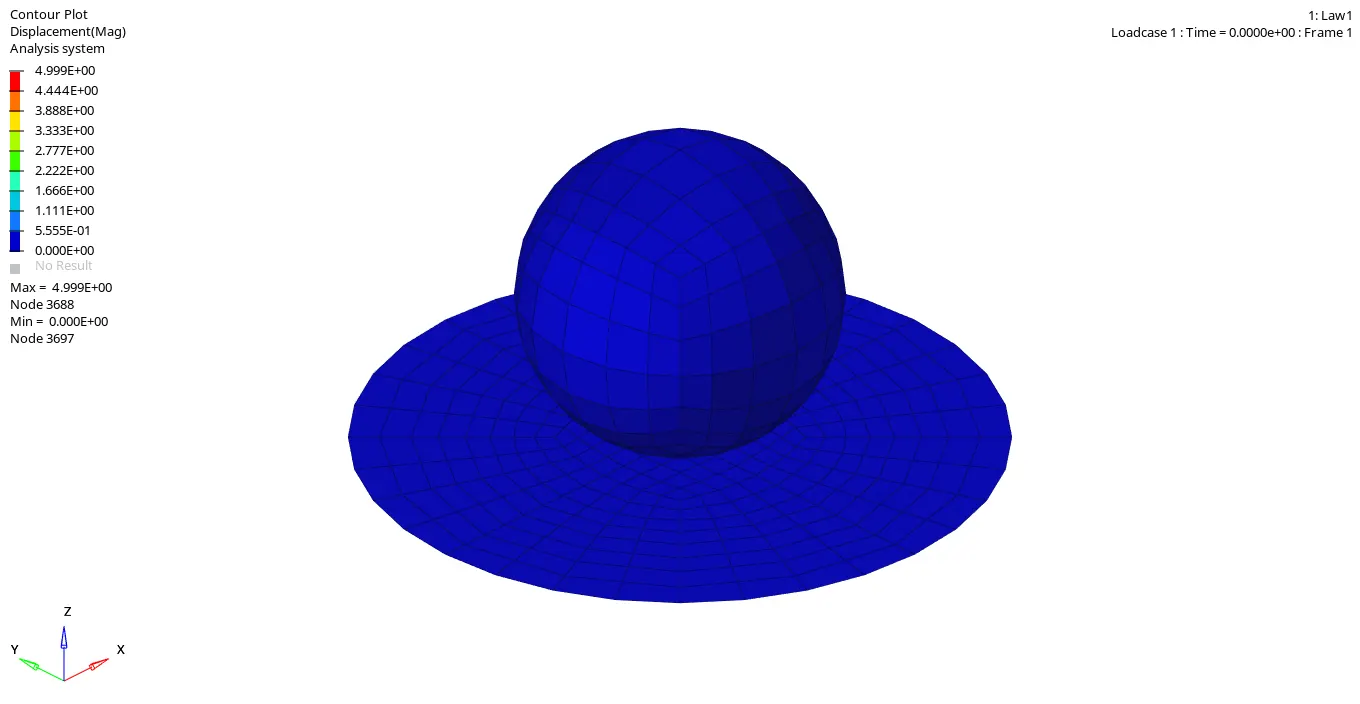
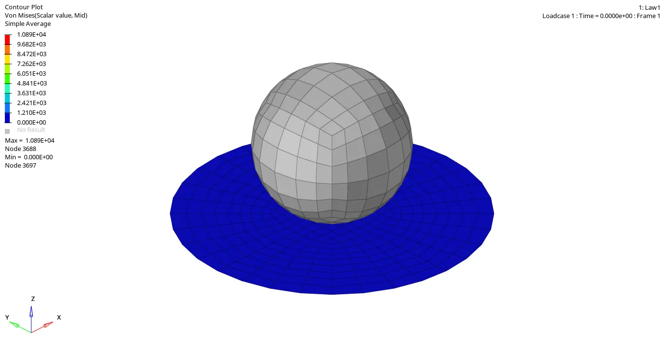
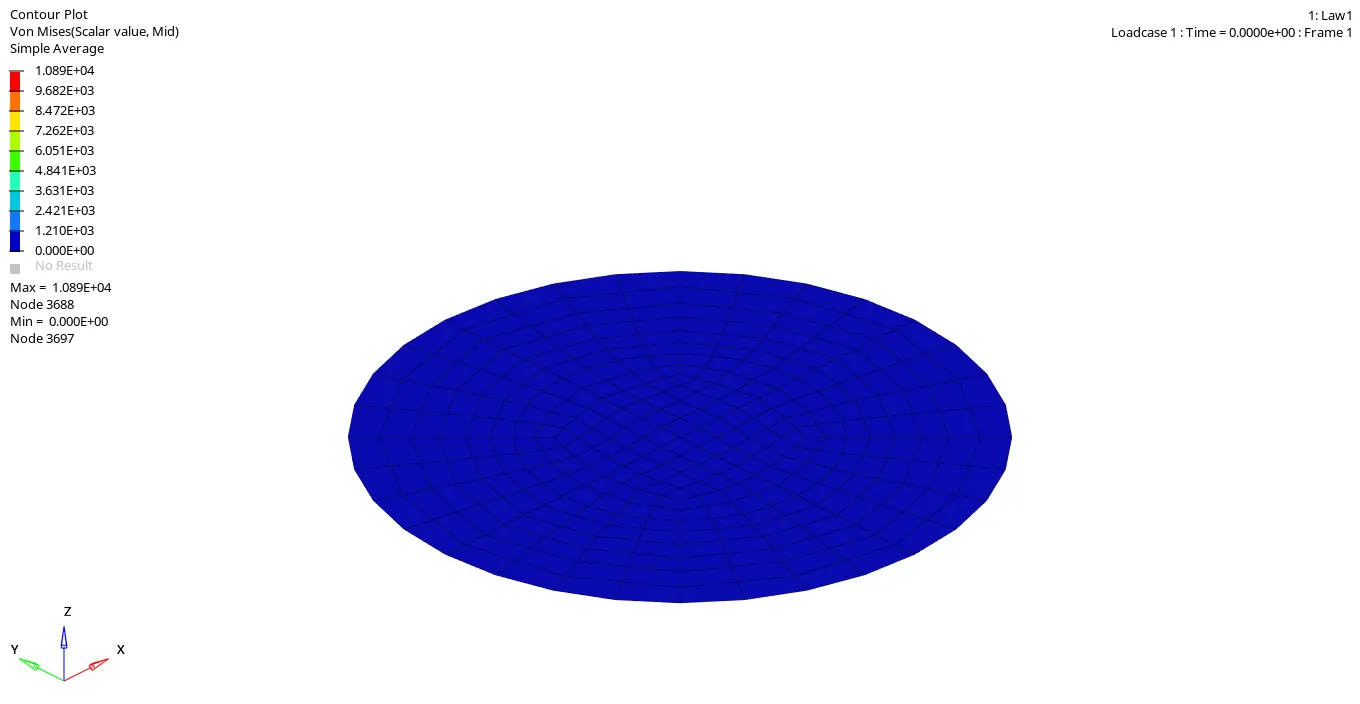
From the simulation results, it was observed that the maximum displacement experienced by the plat elements before getting deleted was around 4.99 mm while the maximum stress generated on the plate was around 10890 MPa.
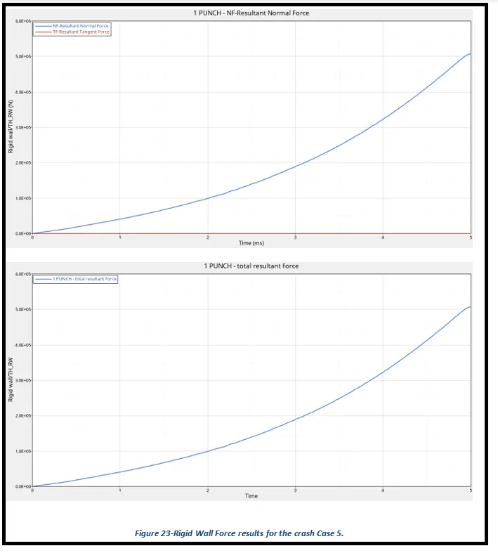
The rigid wall forces are generally the forces experienced by the wall during a crash test. For the challenge purposes, the Total Resultant Force graphs were plotted for both the crash test analysis. From Figure 23, it can be seen that the Net Resultant Normal force of the rigid wall is exactly identical to the Net Resultant Force of the rigid wall. It can also be seen that the Net Resultant force and Resultant Normal force both increase constantly throughout the simulation. This has been the result of using the LAW 1 Elastic Material card.
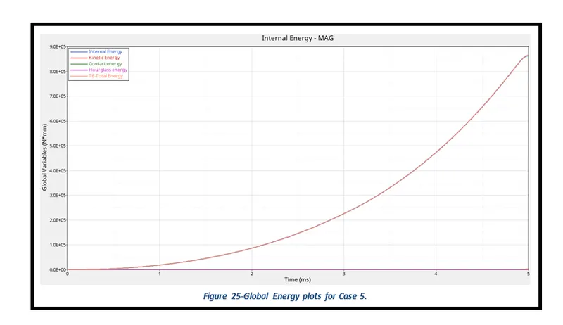
The Total Energy reported by Global variables in Radioss is the sum of internal energy, kinetic energy, contact (sliding) energy, hourglass energy system, damping energy, and rigid wall energy. What can be interpreted from Figure 25 is that the Kinetic Energy, Internal Energy, and Total Energy of the system increase constantly. In addition, it can be observed that the Contact and Hourglass Energy remains constant and negligible.
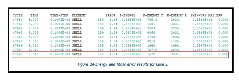
The Energy error should be negative and decrease with the iterations. Thus, ideally, the error should be at most -15% and better to have 5%. The closer to 0% error the better. The Mass error of less than 2% is preferred for the crash simulations. From Figure 24, it can be noted that the simulation yields an Energy Error of 1.3% while the Mass error generated by the simulation for this case is 0%.
Case 6: Law 27 Plas_ Brit Material
The simulation for Case 6 is performed using the same process that was used for Case 4. However, the LAW27_0000.rad starter file was used for this case.
Case 6- Law 27 Plas_Brit Material Simulation Results
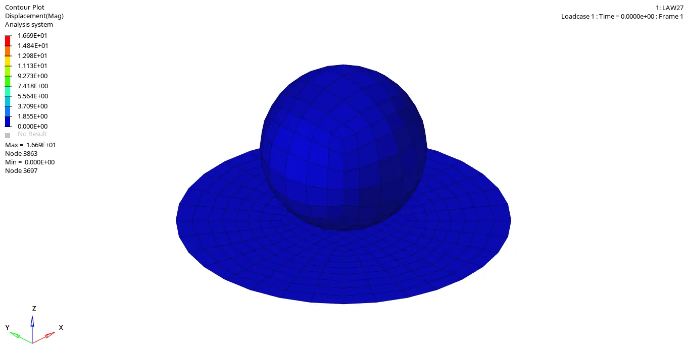
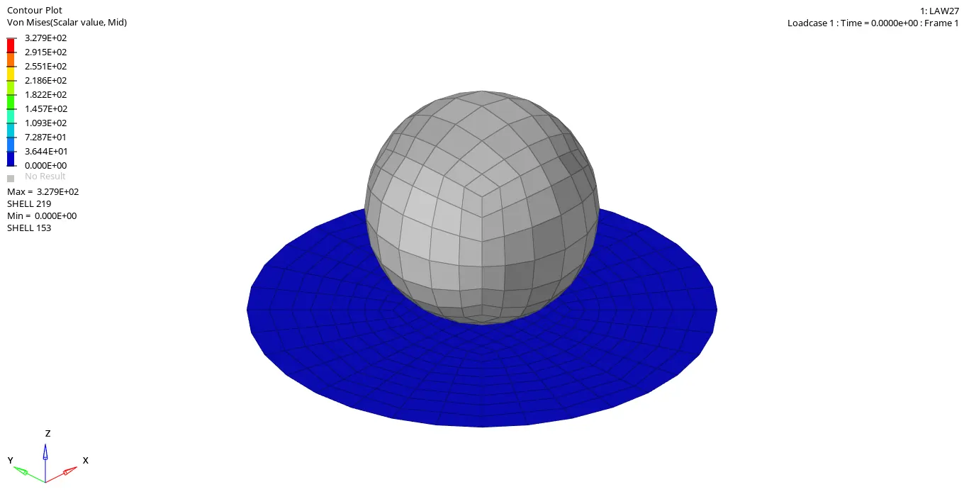
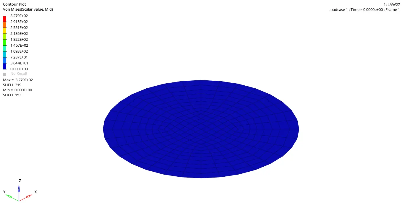
From the simulation results, it was observed that the maximum displacement experienced by the plat elements before getting deleted was around 16.7 mm while the maximum stress generated on the plate was around 327.9 MPa.
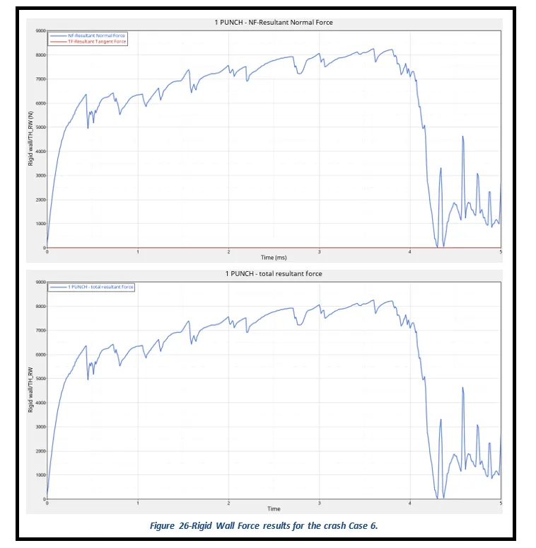
The rigid wall forces are generally the forces experienced by the wall during a crash test. For the challenge purposes, the Total Resultant Force graphs were plotted for both the crash test analysis. From Figure 26, it can be seen that the Net Resultant Normal force of the rigid wall is exactly identical to the Net Resultant Force of the rigid wall. It can also be seen that the Net Resultant force continuously increases between 0 to 4 ms and then it drops significantly and varies a bit and becomes 0 at the end of the simulation. The drops in the magnitude of resultant forces have essentially occurred due to the deletion of the elements.
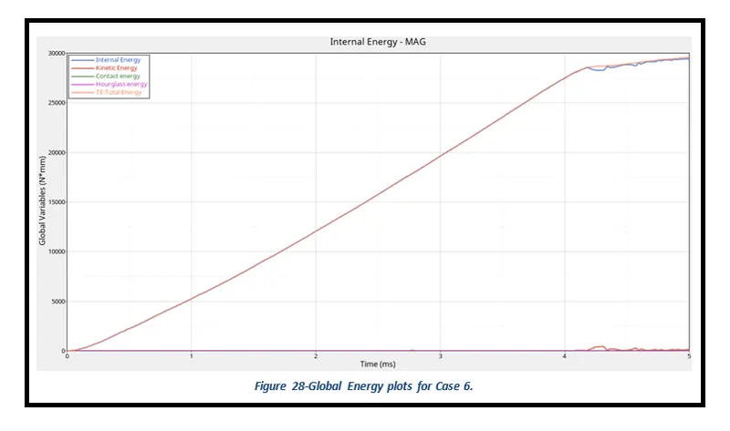
The Total Energy reported by Global variables in Radioss is the sum of internal energy, kinetic energy, contact (sliding) energy, hourglass energy system, damping energy, and rigid wall energy. What can be interpreted from the Figure 28 is that the circular plate resists the motion of the rigid sphere until 4.3 ms and after that, the plate gets ruptured completely by it. Thus, proving that both the kinetic and internal energy increases up to the value of 28675 N*mm, and as soon as the plate allows the sphere to pass through both the energies become almost constant.
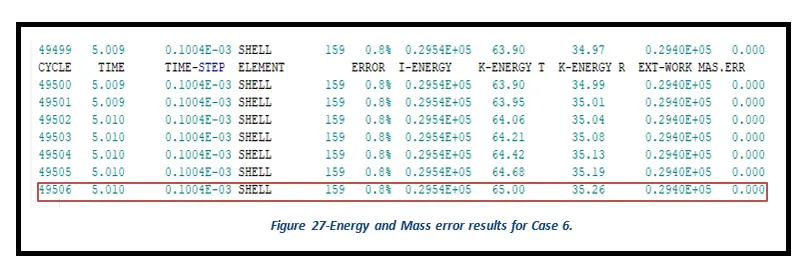
The Energy error should be negative and decrease with the iterations. Thus, ideally, the error should be at most -15% and better to have 5%. The closer to 0% error the better. The Mass error of less than 2% is preferred for the crash simulations. From Figure 27, it can be noted that the simulation yields an Energy Error of 0.8% while the Mass error generated by the simulation for this case is 0%.
Case 7: Law 36 Elasto Plastic Material
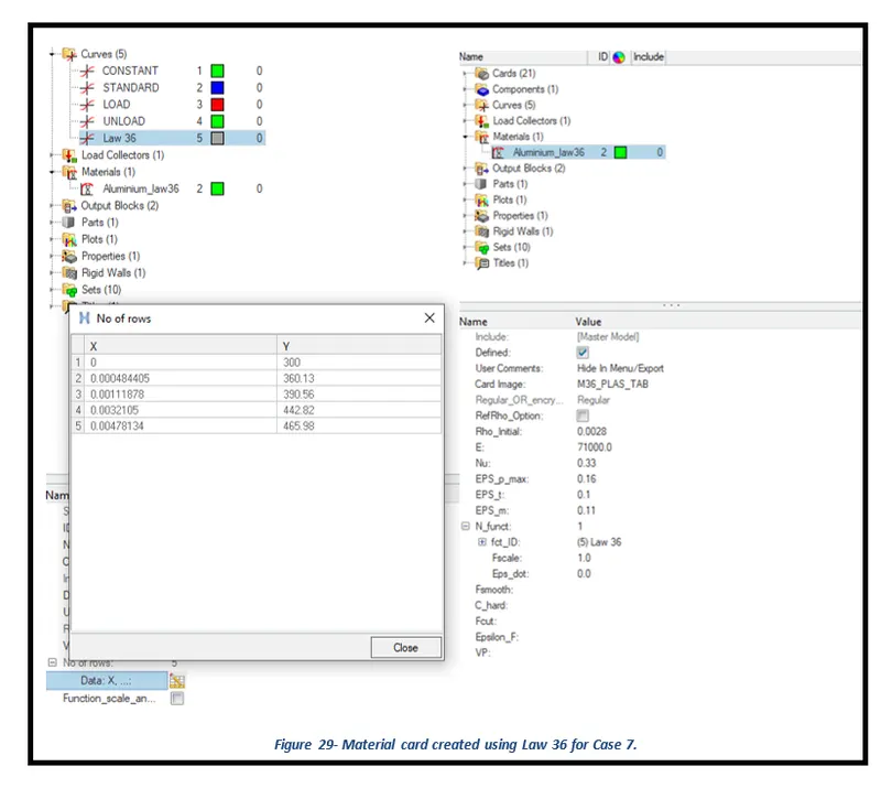
The simulation for Case 7 is performed using the same process and the same starter file that was used for Case 6. However, Material card LAW 36 was used for this case and the engineering stress-strain date used for the material card is presented in the following figure.
Case 7- Law 36 Elasto Plastic Material Simulation Results
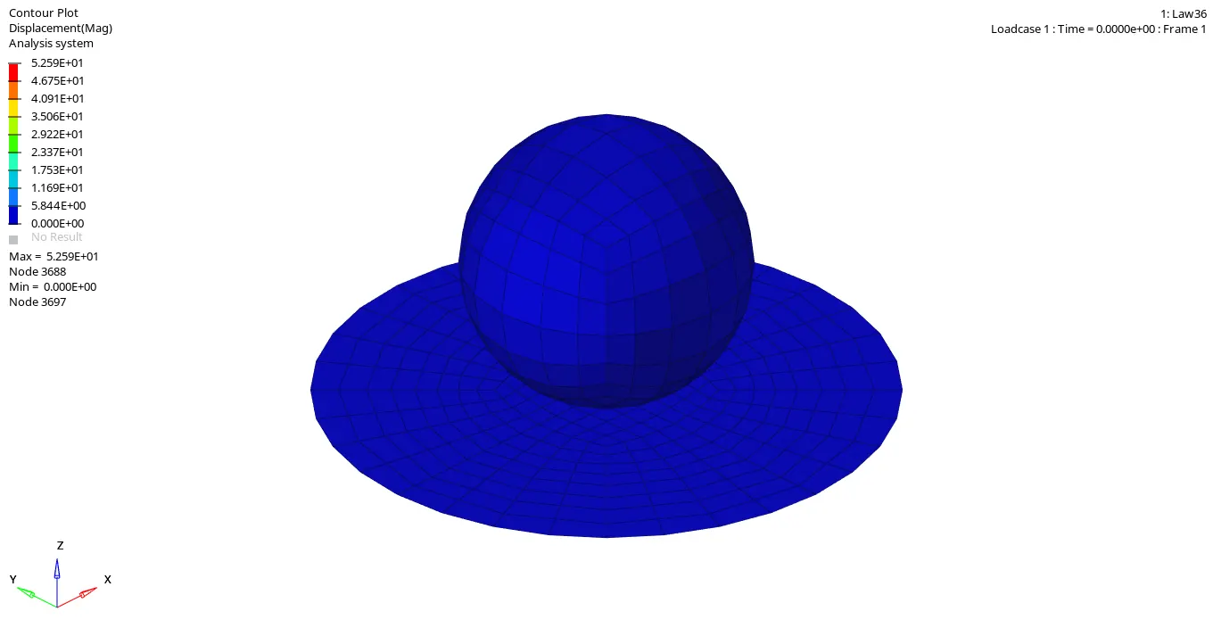
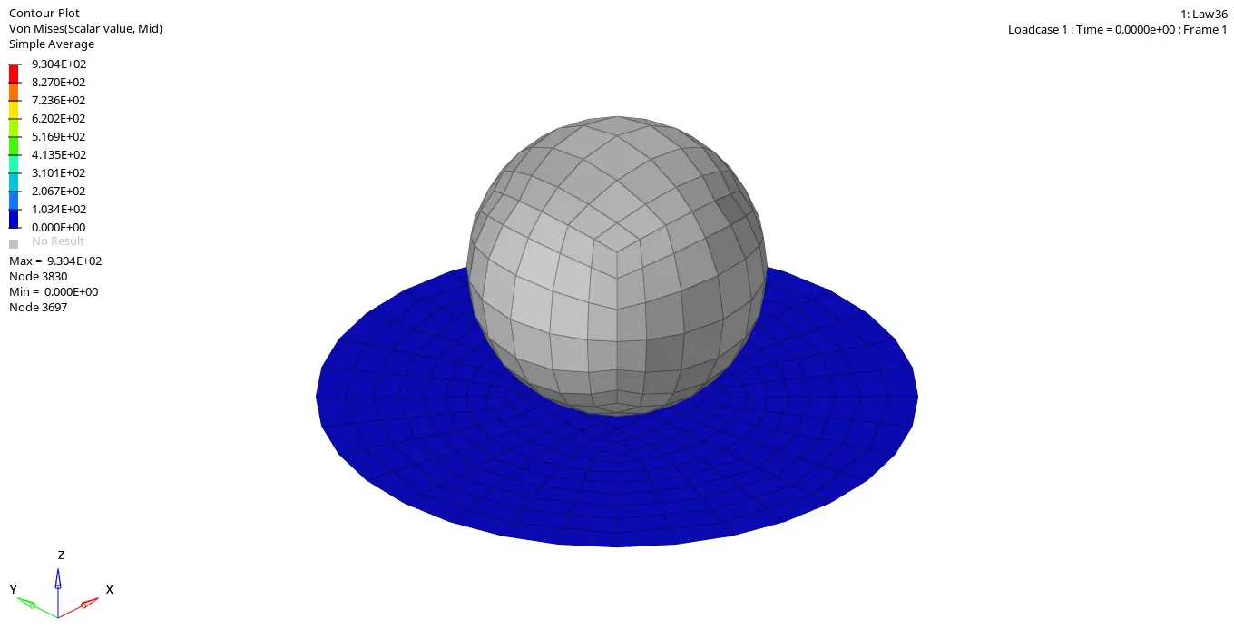
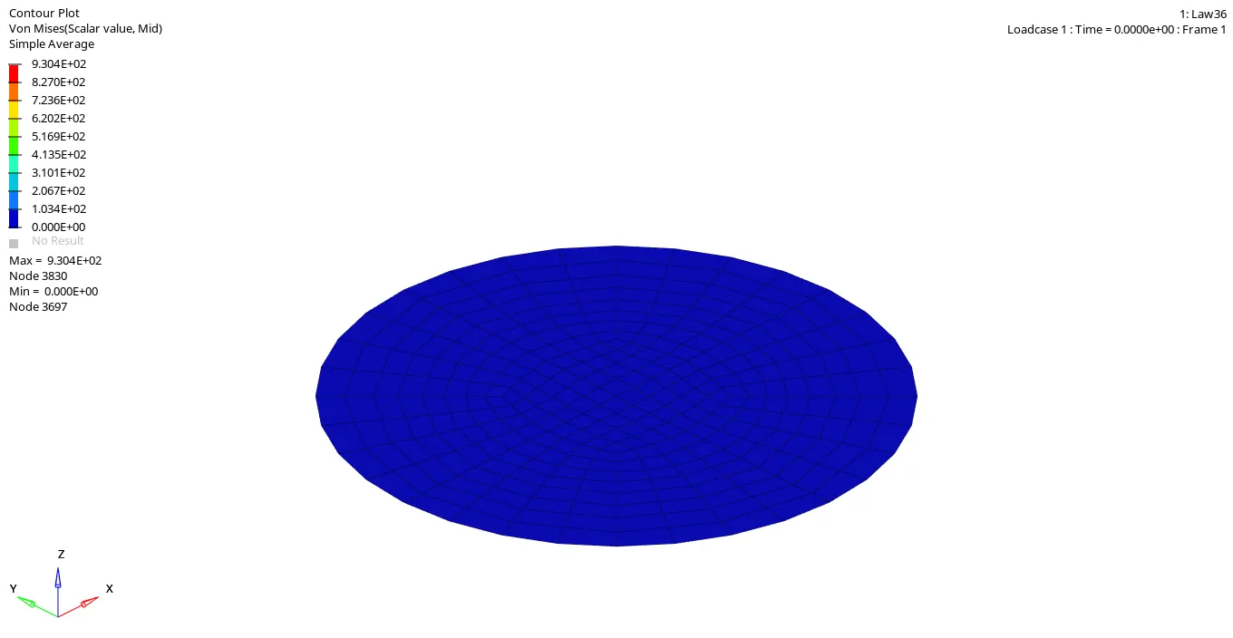
From the simulation results, it was observed that the maximum displacement experienced by the plat elements before getting deleted was around 52.6 mm while the maximum stress generated on the plate was around 930.4 MPa.
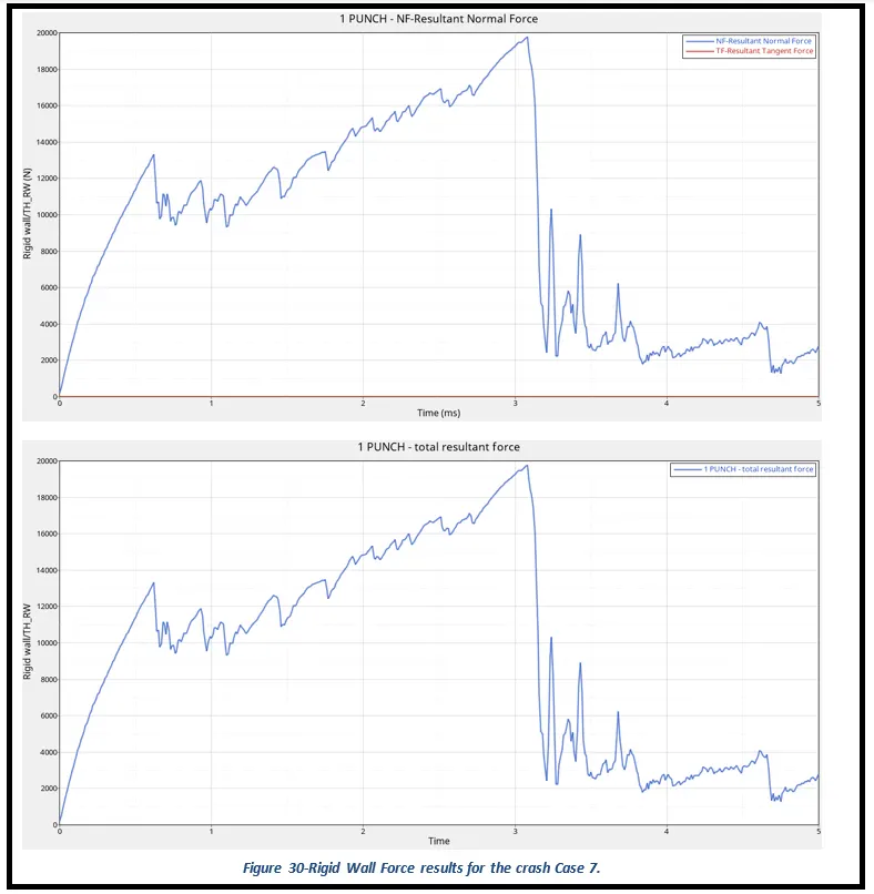
The rigid wall forces are generally the forces experienced by the wall during a crash test. For the challenge purposes, the Total Resultant Force graphs were plotted for both the crash test analysis. From Figure 30, it can be seen that the Net Resultant Normal force of the rigid wall is exactly identical to the Net Resultant Force of the rigid wall. It can also be seen that the Net Resultant force continuously increases between 0 to 3.1 ms and then it drops significantly and again shoots up and varies till the end of the simulation. The drops in the magnitude of resultant forces have essentially occurred due to the deletion of the elements.
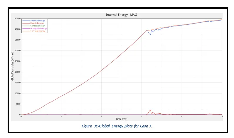
The Total Energy reported by Global variables in Radioss is the sum of internal energy, kinetic energy, contact (sliding) energy, hourglass energy system, damping energy, and rigid wall energy. What can be interpreted from Figure 31 is that the circular plate resists the motion of the rigid sphere until 3.16 ms and after that, the plate gets ruptured completely by it. Thus, proving that both the kinetic and internal energy increases up to the value of 44350 N*mm, and as soon as the plate allows the sphere to pass through both the energies become almost constant.
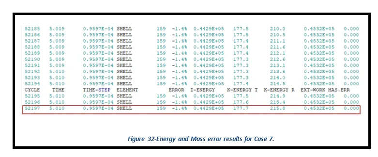
The Energy error should be negative and decrease with the iterations. Thus, ideally, the error should be at most -15% and better to have 5%. The closer to 0% error the better. The Mass error of less than 2% is preferred for the crash simulations. From Figure 32, it can be noted that the simulation yields an Energy Error of -1.4% while the Mass error generated by the simulation for this case is 0%.
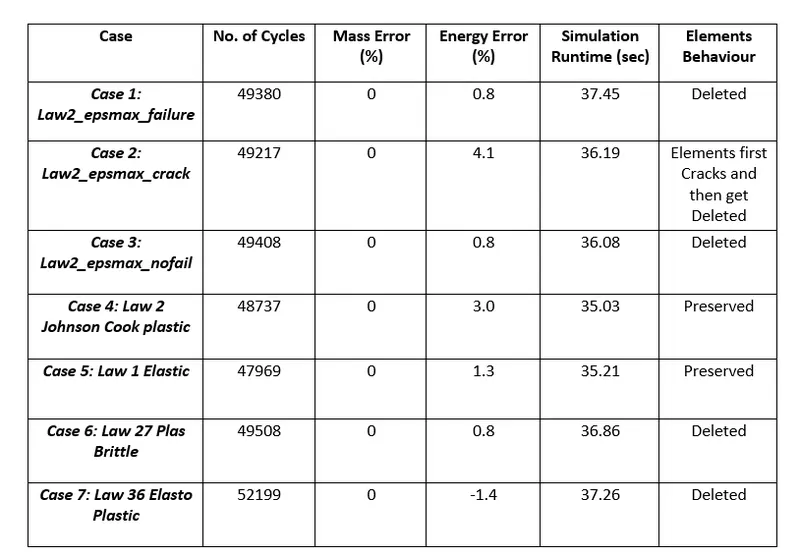
Summarization of the Results of 7 different cases
4 Conclusion
In conclusion, the main aim of assignment 4 was to perform crash simulations of the given Circular plate model using seven different Material Laws. Perform mass and energy error checks and determine whether the results are acceptable. Lastly, plot rigid wall forces and global energy plots and compare the obtained results for the same.
After performing the simulations for all the cases, it was found the elements in cases 1, 3 6, and 7 gets deleted as soon as the solid sphere hits the circular plate. In case 2, it was observed that first the crack develops between the elements, and then the elements get deleted as soon as the stress within the plate exceeds that of the failure criterion defined for the material card. However, the elements in cases 4 and 5 remain preserved as there is no failure criterion defined for their respective material cards.
Considering the above-discussed aspects of the simulations, it would not be wrong to say that Case 2 presents the best on-field scenario for the crash simulation of a Circular Aluminium plate.