Plate Simulation

AIM:

Simulate with various parameters and compare the results with different plot graphs.

METHODOLOGY:

• Import the geometry.
• Set the boundary conditions.
• Run the simulation.

PROCEDURE:

Importing:

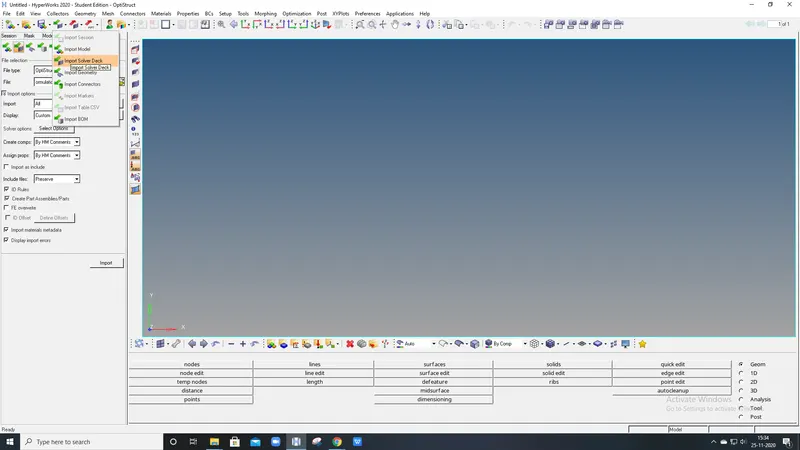
• To open .rad file, Go to the Import option in the Standard tool bar.
• Select Import as Solver Deck and select the file.
• Click on Import.

Simulation:

Case 1:

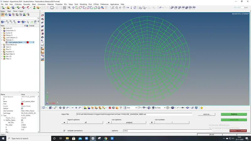
• Open the material card in the tab area.
• Change the card name to Law2_epsmax_failure.
• Click on RADIOSS in the Analysis panel.
• Browse the file and and click on save as.
• Create a new folder and tick the include connectors
• Type as “-nt 4” in the options bar and click on Radioss.
• Run the simulation.

Case 2:

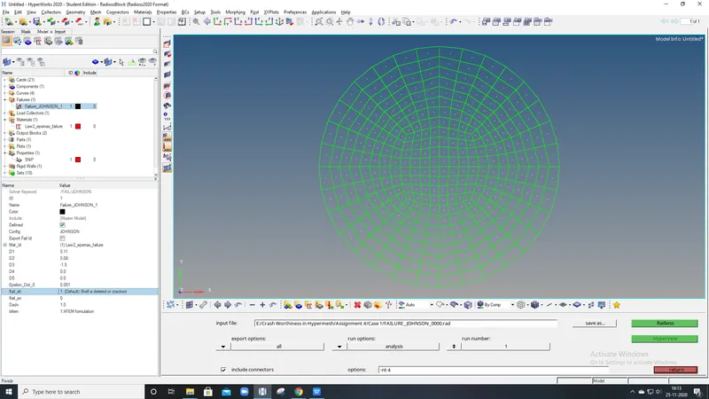
• Open the Failure card named as Failure_JOHNSON_1.
• Change the parameters Ifail_sh, Dadv and Ixfem as 1,1,1 respectively.
• Again open the material card and rename it as Law2_epsmax_crack.
• Click on RADIOSS in the Analysis panel.
• Browse the file and and click on save as.
• Create a new folder and tick the include connectors
• Type as “-nt 4” in the options bar and click on Radioss.
• Run the simulation.

Case 3:

• Delete the Failure card by right clicking and selecting the Delete option.
• Select the material card and again rename as Law2_epsmax_nofail.
• Click on RADIOSS in the Analysis panel.
• Browse the file and and click on save as.
• Create a new folder and tick the include connectors
• Type as “-nt 4” in the options bar and click on Radioss.
• Run the simulation.

Case 4:

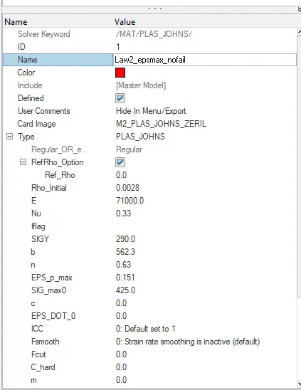
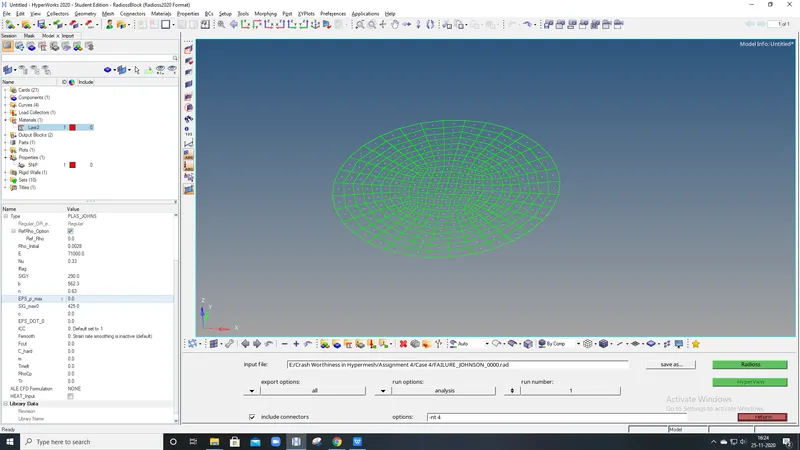
• Open the material card and change the card name to Law2.
• Check the parameters and Change the Eps_p_max value to “0”.
• Click on RADIOSS in the Analysis panel.
• Browse the file and and click on save as.
• Create a new folder and tick the include connectors
• Type as “-nt 4” in the options bar and click on Radioss.
• Run the simulation.

Case 5:

• Open the material card and change the card name to Law 1 Elastic.
• Change the parameters like Rho_Initial,Young’s Modulus E, and Possion’s ratio Nu as 0.0028,71000 and 0.33 respectively.
• Rename material card name as Law 1.
• Click on RADIOSS in the Analysis panel.
• Browse the file and and click on save as.
• Create a new folder and tick the include connectors
• Type as “-nt 4” in the options bar and click on Radioss.
• Run the simulation.

Case 6:

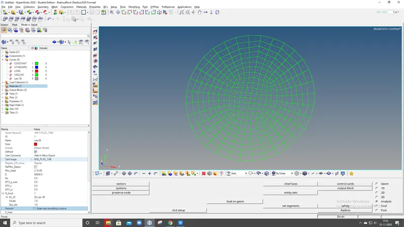
• Change to Law 36 in card name located in the material card.
• Rename material card name to Law36.
• Set the required parameter values.
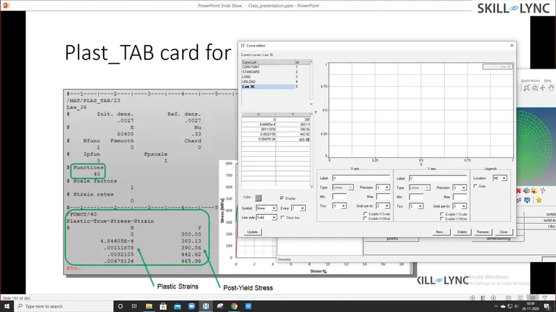
• Curve should be created to specify the fct_ID.
• Create a curve in model browser and plot the values by clicking the new curve.
• Open the material card assign the curve in fct_ID parameter.
• Click on RADIOSS in the Analysis panel.
• Browse the file and and click on save as.
• Create a new folder and tick the include connectors
• Type as “-nt 4” in the options bar and click on Radioss.
• Run the simulation.

Case 7:

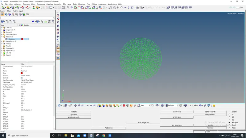
• Change the card type to Law 27 and rename it as same.
• Check the parameters values with the given values.
• Click on RADIOSS in the Analysis panel.
• Browse the file and and click on save as.
• Create a new folder and tick the include connectors
• Type as “-nt 4” in the options bar and click on Radioss.
• Run the simulation

Animations:

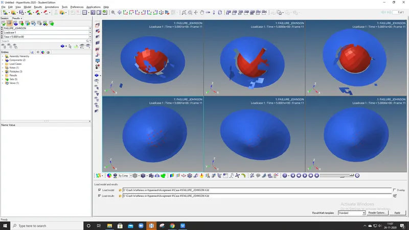
• Select the HyperView in the Client Selector in the toolbar.
• Browse the .h3d files for each case.
• Make sure load file and load results is ticked or selected.
• Click on ‘apply’.

Graphs:

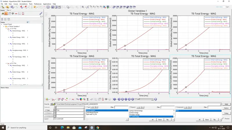
• Select the HyperGraph 2D in the Client Selector located in the toolbar.
• Browse the T01 files for each case.
• Select different energies to compare and click on Apply.

Energies to be compared:

Total Energy:

The total energy of a system is the sum of kinetic and gravitational potential energy, and this total energy is conserved in orbital motion. Objects must have a minimum velocity, the escape velocity, to leave a planet and not return.

Internal Energy:

The internal energy of a thermodynamic system is the energy contained within it. It is the energy necessary to create or prepare the system in any given internal state.

Contact Energy:

The frictional energy (FE) is already included in the slave energy (SE) and the master energy (ME) and hence also in the sum of slave/master energy (SoSM). Thus, one gets the energy needed to prevent penetration between the contact partners by subtracting the frictional energy (FE) from the sum of slave/master energy (SoSM). In the absence of friction the slave energy (SE) and the master energy (ME) should be close in magnitude but opposite in sign and the sum of slave/master energy (SoSM) should equal the stored energy.

Hourglass Energy:

Hourglass (HG) modes are nonphysical, zero-energy modes of deformation that produce zero strain and no stress. Hourglass modes occur only in under-intetgrated (single integration point) solid, shell, and thick shell elements. LS-DYNA has various algorithms for inhibiting hourglass modes. The default algorithm (type 1), while the cheapest, is generally not the most effective algorithm.

Definations:

Ixfem:

Ixfem cracks the elements instead of deleting the element. It is used only for shell elements.

Eps_p_max:
Maximum strain where elements starts to get cracked or deleted.

Dadv:

It is criterion for crack advancements.

Comparison:

Case 1,2,3:

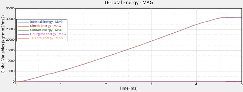
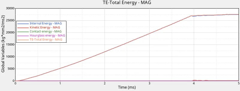
• Total Energy and Internal Energy varies linearly in three cases. But there is slight deflection in the ending time.
• There is slight deflection in kinetic energy when internal energy is deflected.
• Hourglass energy, Contact energy are constant throughout the process in all cases.
• This is due to Ishell parameter set to 24 in which it minimes the hourglass energy.
• In case 2, the elements deleting or cracking are less due to Dadv parameter.

Case 1

Case 2

Case 3

Case 4,5,6:

• Total Energy and Internal Energy are varying linearly in case 4&6. But in case 5 they are varying exponentially.
• This exponentially varying is due to pure elastic nature material in case5.
• Hourglass energy, Contact energy are constant in all the cases.
• Kinetic energy is constant in case 4 & 5 cases, but in case 6 there is deviation in the curve.
• When compared to case 1,2,3 and 6, in case 6 kinetic energy deviation is more.
• In case 5 there is will be no element deletion or cracking due to pure elastic material.

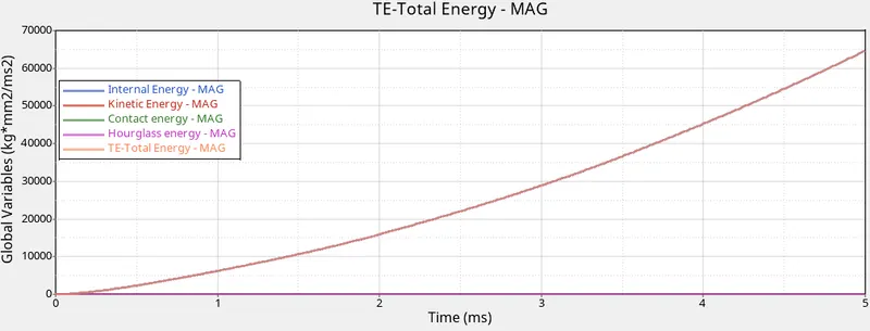
Case 4

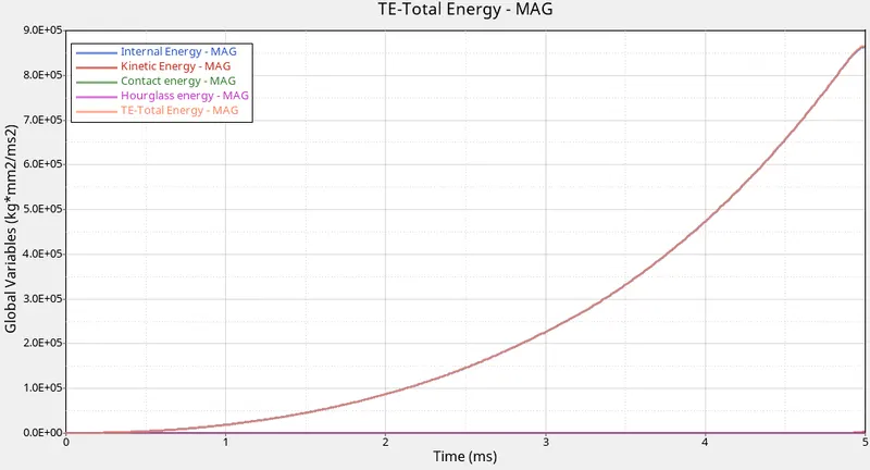
Case 5

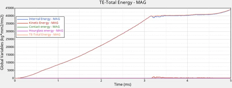
Case 6

Learning Outcome:

• Different types of materials like

Law 1 Elastic

Law 2 Johnson Cook

Law 27 Elasto Plastic

Law 36 Elasto Plastic Tabulated

Law 42 Ogden

Law 70 Foam

• Parameters definations like

Ixfem

Dadv

Dmax

Ifail_sh etc

RESULT:

Case 4 is most preferable or suitable material for this rupture plate due to its application.

In case 4, Law 2 Johnson Cook material is suitable due to its own parameters values.

If elements should be deleted and hit the surface then Law 27 is preferable.

Case 4