Assignment 3

Aim:

The main goal is to complete the given tasks which are given to simulate the given model with a different set of parameters. The task given is as follows

Questions:

Comparison of results with base simulation and improved shell element properties

1. Using the crash beam file from the previous assignment, change the run time to 55 ms.

2. Change the number of animation steps during simulation to a minimum of 25 and a maximum of 60.
3. Run the base simulation without any modification to element properties.
4. At the end of the simulation, do the energy error and mass error checks and determine whether the results would be acceptable.
5. If acceptable, Plot rigid wall forces, internal energy, hourglass energy, contact energy, total energy of the simulations.
6. Change all the shell elements properties to recommended properties, save this as separate, rad files, and run the simulation.
7. Follow steps 5 and 6.
8. Create a brief report comparing all the results from steps 5 and 6 for both simulations.
9. Comment whether there is any change in the results and why there is any change in the result.

Methodology:

The process which is followed is written below.

1. Opening the file
2. Changing the Run Time
3. Changing the Simulation Step
4. Changing the Properties.
5. Simulation Changes
6. Opening Hyper View
7. Opening HyperGraph

Procedure:

Case 1: (Default Properties)

1. Opening the File:

• The Model is not in .hm format therefore there are other steps to follow to open the file.
• To open the file, Click Import Solver Deck in the Toolbar >> Select the Starter File ( Starter File does end with 0000.rad Ex: XXXX_0000.rad) >> Click Import.
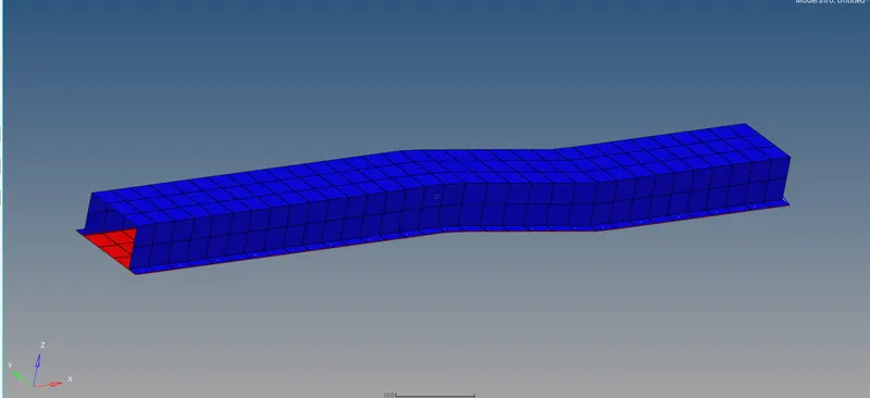
• The File is imported and the model is displayed on the Graphics Area.

2. Changing the Run Time:

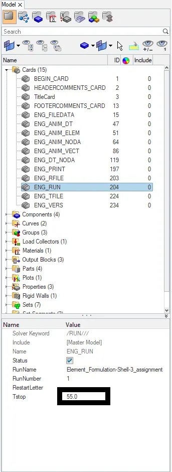
• The run time needs to be changed to 55ms (as per question). To change the run time, the following steps can be followed.
• Go to the Model Browser in the Tab Area, Click on Cards dropdown >> Select ENG_RUN >> A page is display in the Entity Editor (Found Just below the Tab Model Browser and in the Tab Area reason) >> Change the Tstop value to 55.
• The Value gets changed to the given input I.e. 55.

3. Changing the Simulation steps:

• Similar Steps are used for the simulation of the Model.
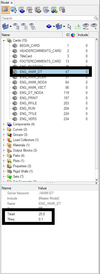
• Go to the Model Browser in the Tab Area, Click on Cards dropdown >> Select ENG_ANIM_DT >> A page is display in the Entity Editor (Found Just below the Tab Model Browser and in the Tab Area reason) >> Change the Tstart value to 25. (optional: change the Tfreq to 0.1 - it simulates the 300 frames per second. If kept as 1 - it simulates 30 frames per second)
• The Value is changed now the Shell Element Formulation needs to be done.

4. Simulation changes:

• The files and the data are needed to be stored in a particular local variable. For the simulation to run smoothly, the files need a location to save.
• Go to the Analysis panel >> Click on Radioss >> Select the File to open. The File that needs to be opened is a starter file. >> Check the Include connectors >> Enter “-nt 4” in the options blank >> Click Radioss.

5. Opening HyperView:

• To Open the HyperView Window, go to the Client Selector in the toolbar >> click on the Hyper View option >> the HyperView Tab opens.
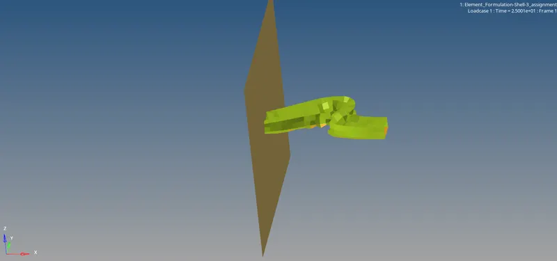
• Once the HyperView is opened, A New Panel is seen >> Browse on the Load model >> Select the .H3D file ( Since the .h3d file has all the simulation frames combined in it) >> Click Apply.

6. Opening HyperGraph:

• To open HyperGraph, On the Client Selector in the Tool Bar, Select HyperGraph 2D >> The HyperGraph opens
• Once the HyperGraph is opened, In the Panels Area, Select the Data File ( the Data File have T01 at the end of the name. ) >> Click Apply >> In Y Type, Select Global Variables >> In Y request, Select Internal Energy >> In Y component, Select MAG >> Click Apply.

• The Above Process is similar for the Contact Energy, Hourglass Energy, and the Total Energy. (Note: all these are in Global Variables)
• For the Rigid Wall Forces, Select the Rigid wall/ Rwall-force on Y Type >> Select 4 RIGID WALL 1 in Y request >> Select total resultant force in Y component. >> click Apply.
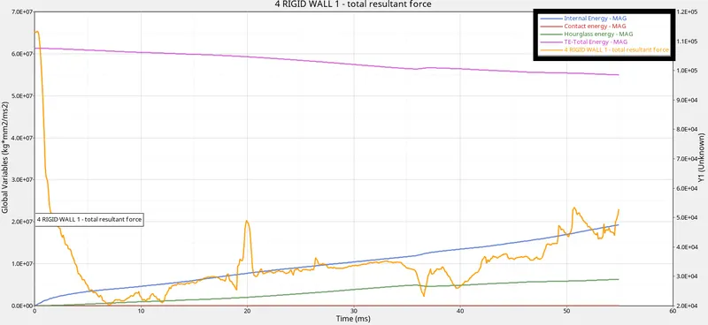
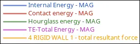
• The Graphs are created for the default property cases.

`darr`

Case 2: (Adding Property)

The Case is similar to that of case 1. In this case, we’re setting the property criteria so that to check which is sustaining less deformation and which method is better for the model.

1. Opening the File:

• The Model is not in .hm format therefore there are other steps to follow to open the file.
• To open the file, Click Import Solver Deck in the Toolbar >> Select the Starter File ( Starter File does end with 0000.rad Ex: XXXX_0000.rad) >> Click Import.
• The File is imported and the model is displayed on the Graphics Area.
• The File opened is the same as the previous overwritten file.

2. Changing the Properties:

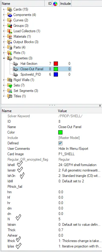
• The properties can be changed on the Model Browser. Go to the model browser in the Tab Area >> Select Properties >> Check for the properties and the Property card image should be ‘P1_SHELL’ >> In the Entity Editor, change the Ishell, Ismstr, Ish3n, N, Ithick, Iplas values as given
• Ishell = 24, Ismstr =2, Ish3n =2, N=5, Ithick=1, Iplas=1 (the values should be entered)
• The property values are changed.

3. Simulation changes:

• The files and the data are needed to be stored in a particular local variable. For the simulation to run smoothly, the files need a location to save.
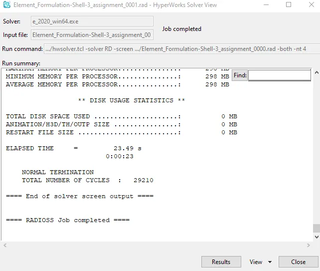
• Go to the Analysis panel >> Click on Radioss >> Select the File to open. The File that needs to be opened is a starter file. >> Check the Include connectors >> Enter “-nt 4” in the options blank >> Click Radioss.

4. Opening HyperView:

• To Open the HyperView Window, go to the Client Selector in the toolbar >> click on the Hyper View option >> the HyperView Tab opens.
• Once the HyperView is opened, A New Panel is seen >> Browse on the Load model >> Select the .H3D file ( Since the .h3d file has all the simulation frames combined in it) >> Click Apply.

5. Opening HyperGraph:

• To open HyperGraph, On the Client Selector in the Tool Bar, Select HyperGraph 2D >> The HyperGraph opens
• Once the HyperGraph is opened, In the Panels Area, Select the Data File ( the Data File have T01 at the end of the name. ) >> Click Apply >> In Y Type, Select Global Variables >> In Y request, Select Internal Energy >> In Y component, Select MAG >> Click Apply.
• The Above Process is similar for the Contact Energy, Hourglass Energy, and the Total Energy. (Note: all these are in Global Variables)
• For the Rigid Wall Forces, Select the Rigid wall/ Rwall-force on Y Type >> Select 4 RIGID WALL 1 in Y request >> Select total resultant force in Y component. >> click Apply.
• The Graphs are created for the default property cases.

Result:

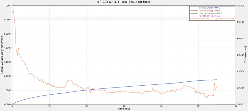
The Simulation for the model is completed and the graph is plotted for the given file.

Observations:

Both the cases are simulated and the plots are given for these. The observations are seen are below.

Case- 1:

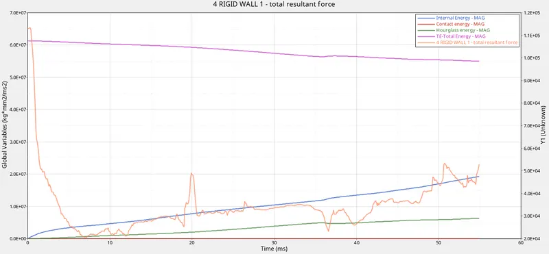
Case- 2:

We can see from the above graphs that Hourglass Energy is changing from case 1 to 2 and the Total Energy also changes from case 1 to 2.

We know that if the Total Energy is constant in the 2nd graph which says that there is no fluctuation of the energy. therefore strain deformation reduces a bit.

The Hourglass Energy became zero in the `2^(nd)` case which mean the Model has a minimum stiffened response

Terms used:

Tstart:

Tstart is the Time at which the Simulation Starts.

Tstop:

Tstop is the Time at which the Simulation stops.

Ishell:

Ishell is an Element Formulation for the 4 noded shells.

Ismstr:

Ismstr is an Element Formulation for the Small or Large strains

Ish3n:

It is an Element Formulation for 3 noded shells.

Integration Points:

An FE solver computes displacement and force results at the element nodes. The shape function is used to interpolate the nodal results onto the interior of the element. Unlike displacements and forces, strains and stresses are not computed at the nodes. They are computed at specific integration points within the element.

Ithick:

To determine if the thickness must be remained constant or does it have a varying thickness

Iplast:

It is used for calculating post-yield strain

HourGlass Energy:

Hourglass modes are nonphysical modes of deformation that occur in under integrated elements and produce no stress.

• Solid elements with a single integration point. Shell or Tshell elements with a single in-plane integration point.
• One point integration is much faster so we usually tolerate, but try to minimize hourglass modes.

Reduced integration can lead to non-physical zero-energy modes called hourglass modes.

Hourglassing can usually be controlled by applying internal forces to resist hourglass modes via one of several HG control algorithms. Hourglass energy, which is work done by the forces calculated to resist hourglass modes, takes away from the physical energy of the system.

There are two methods used to control the formation of hourglassing

1. Perturbation:

• The hourglass deformation is detected with the relative motion (Velocity) of the nodes.
• When hourglassing is detected, a force is applied on the node to stabilize the deformation.
• This force is defined according to the element stiffness (Young's Modulus, yield stress, Plastic, etc)
• This force introduces artificial energy.

2. Physical Stabilization

• Hourglass yield depends on the natural yield.
• Hourglass loading stiffness depends on the natural tangent modulus.
• The hourglass treatment is done at the material level.

The elements may have bad behavior in the case of large rotation and distortion and in the case of elastic loading and unloading cycles.