Assignment 3-2D Element Formulation Challenge

Objective: compare the results of simulations with and without recommended properties, do energy and mass error checks, plot graphs for rigid wall forces, Internal energy, hourglass energy, contact energy and total energy

Given data:

1. change the run time to 55 ms.

2. change animation steps during simulation in between 25 minimum and maximum 60.

Recommended properties:

Ishell =24

QEPH 4 nodes shells are the best combination of cost and accuracy.

it is an improved under-integration scheme, has 1 integration point on the surface at the centre, it takes less time for computation compared to a 4-point integration scheme and has a major advantage as it stabilizes the hourglass mode.

Hourglass mode:

Hourglass modes are nonphysical modes of deformation that occur in under-integrated elements and produce no stress.

Ismstr =2

Large strain with full geometric nonlinearities

for problems with large displacements and strains where large deformations occur in less time, this scheme helps to give better accuracy. strain is computed based on the current element shape with the derivative of the shape function & small strain activation is possible in the Radioss engine

Ish3n =2

standard 3 nodded shell (co) with modification for large rotation (default)

this scheme has 1 integration point, and it is stabilized against hourglass and take less time

N=5

number of integration points set to 5 for accuracy bending

up to 10 integration points are acceptable through-thickness, recommended N=5 (i.e. 5 integration points throughout the thickness.)

Ithic =1

thickness change is taken into account for accuracy

here change in thickness is not only considered for post-processing but also used to compute the strain and stress from true thickness.

Iplas =1

iterative plasticity for good accuracy

it takes care when stresses go beyond yield stress in the plastic region, it updates strain, thickness and stresses accordingly

Procedure:

Import file

to start we have to import starter file into the radioss environment this can be done by going into task bar >> import >> solver deck

Here we selected 0000.rad file and click import

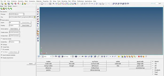
On import file appears as below

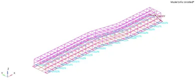
Edit run time and T freq :

To change T stop (total run time) go to model browser >> select card >> ENG_RUN >> at Tstop an input box will be there update this box by 55

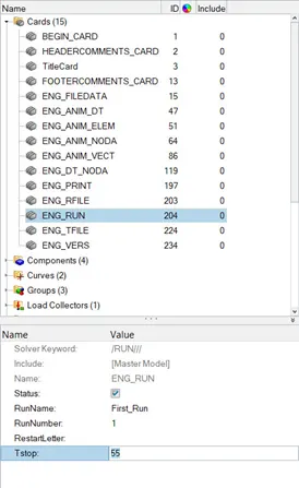
Run Time(T stop)

The run time is total time taken for sound wave to travel through the entire length of model

This can be calculated by formula

Moving to Tfreq (animation frequency)

For here animation steps must be in between 25 to 60.

So we can choose any value in between 25 to 60. for here we are choosing 30

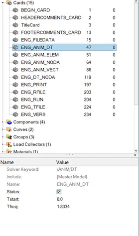
Animation frequency can be calculated by a formula i.e., Run time /number of animation step

Animation frequency = 55/ 30 = 1.8333

To input this value, go to model browser >> select card >> ENG_ANIM-DT >> and input T freq value as 1.8333 as shown below.

CASE 1 -

Run the simulations without any modification to element properties

Now when we import, input run time and animation frequency we can initialize the analysis for that we have to go in analysis panel >> radioss >> input the file: starter file >> radioss

The input file is the same starter file which we had just edited.

Once we hit radioss, a pop-up box will appear it shows us the real time analysis and gives us the final result.

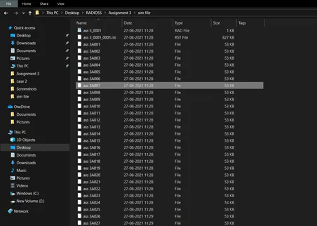
After run it will create multiple files as shown below

At the end of the simulation, do the energy error and mass error checks

The engine output file of 001.out format is generated after analysis; this engine output file contains data during simulation such as:

Cycle time step

Energy error

Mass error

Internal energy

Kinetic energy

Contact energy

Here we have to check for energy and mass error

1.it is normal if error slightly increases

2.the energy error acceptable in the range of -15 % to + 5 %

3.the mass error acceptable in the range of 0 to 2

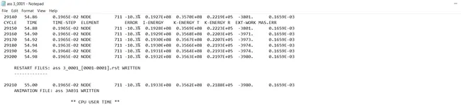
Here we have energy error as -10.3 % and mass error as 0.1659 E-03.

This two are in the acceptable range

But here energy error in increasing because of hourglass

Here the negative sign indicates that there is an energy dissipated from the system or loss of energy

Hyperview Animations

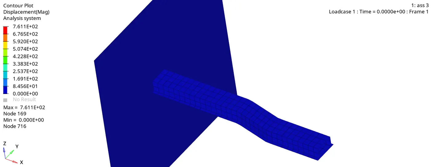
In hyperview we can see where exactly the maximum and minimum values of variable occurs and how exactly model will behave. it is a post processing and visualization environment for FEA that gives the output of the analysis in simulation

To open it select hyperview from selection list in toolbar >> in here there will be two input boxes will be provided select only one of them and chose .h3d file from the file which were created during analysis and click APPLY.

Once model is opened in hyperview environment next stage is to see results such i.e. displacement, von mises or velocity simulation which has to be viewed

To select these, we have to go in contour available in tool bar

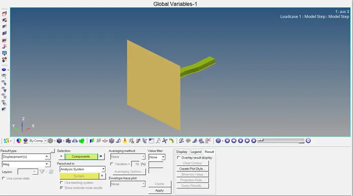
Once respective result is selected (here displacement) click apply and then run the simulation

Plot graph in hypergraph 2D

In radios we can see the graphs of various parameters which gives us better insight of models behaviour. it is a data analysis and plotting tool that represents the FEA from the simulation into graphs with respect to the selected unit system.

To do this first select hypergraph 2D tool from tool selection list available in tool bar >> input the file TO1 generated from radioss

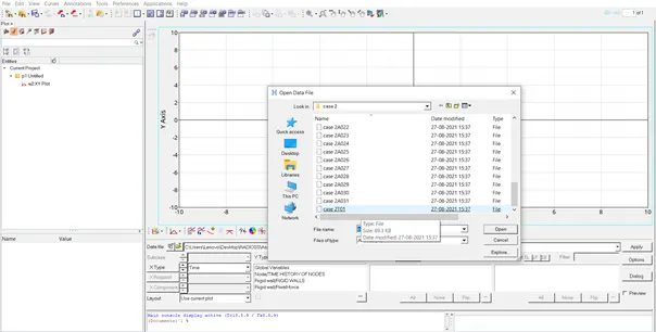
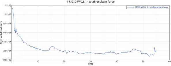
And plat the graph for rigid wall forces as shown below and apply.

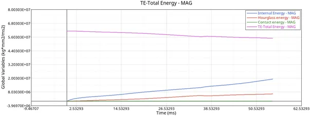
Similarly, for internal energy, hourglass energy, contact energy, total energy

Go to global variable >> internal energy / hourglass energy /contact energy / total energy >> MAG and apply

CASE 2 –

Run the simulation with recommended properties

Once model is being imported in the hypermesh environment go to model browser >> components >> select proper mesh components to be updated by recommended properties as shown below.

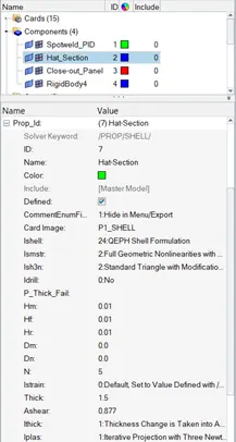
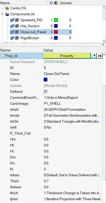
Once updated save the file and do analysis by radioss as done previously

Check energy and mass error for case 2-

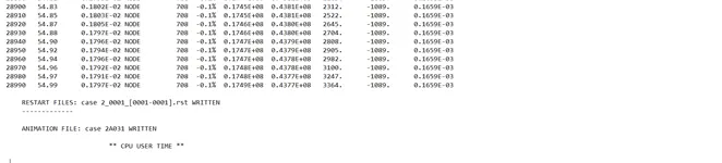
With energy error -0.1 % and mass error 0.1659E-03

Run the simulation with hyperview

Below video shows the animation of how model will deform

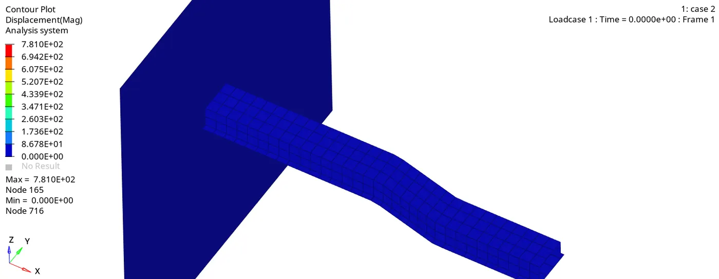
Plot graphs in hyper graph 2D

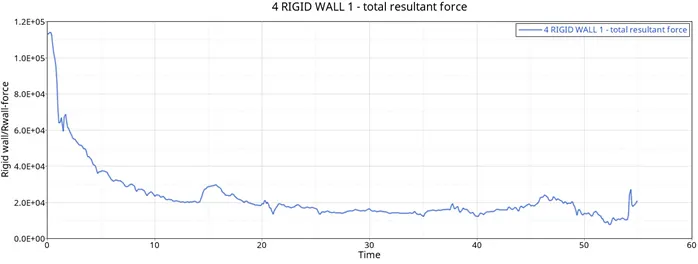
For rigid wall forces graph will be as below

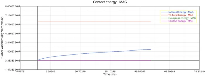
And for internal, contact, hourglass, total energy will be as

Comparison I case 1 and case 2:

Energy and mass error: in case 1 we have energy error as -10.3 % and mass error as 0.1659 E-03. While in case 2 the energy error -0.1 % and mass error 0.1659E-03

We can see here that mass error is remain same while energy error reduces from -10.3% to 0.1 percent. this might be happening because in case 2 total energy and hourglass energy is reduced considerably and we can see that the energy error can be derived from the relation as below

Energy error = hourglass energy + contact energy / total energy

“The result reliability is strongly affected by the energy error percentage; if the error is negative it means some energy has been dissipated, while if positive there is an energy creation.”

As for mass error there is no change in mass for both cases that’s why mass error remains same

Rigid wall / total resultant forces

Case 1-

Case 2 –

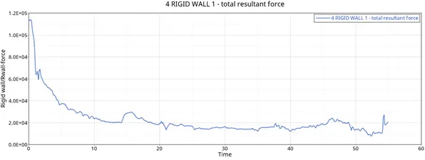
From both above graphs we can see that there is not much difference in the both resultant forces. that is because there is not much difference in external conditions in both the cases. the only difference we made was in the properties of element.

Internal / total / contact/ hourglass energy

Case 1-

Case 2-

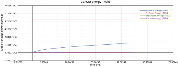
From above graphs we can see that in case 1 total energy line has some downward inclination while in case 2 total energy line is moving straight

This shows that there is no loss of energy happened in case 2

There is slight change in internal energy but not significant

In case 1 we can see the hourglass energy while in case 2 it is completely stabilized

Contact energy is same for both the cases and it remains constant this might be because there is friction less contact happen due to conditions.

Conclusion: from above comparisons we can conclude that with recommended propertied we get more accurate results