Assignment 3-2D Element Formulation Challenge

OBJECTIVES:

Recommended properties:

Parameters		Comment
Ishell =24		QEPH 4 nodes shells are best combination of cost and accuracy.
Ismstr=2		Full geometric nonlinearities (default)with possible small strain formulation activation in RADIOSS Engine.
Ish3n=2		Standard 3 noded shell (C0)with modification for large rotation(default)
N=5		Number of integration points set to 5 for accuracy bending.
Ithick=1		Thickness change is taken into account for accuracy.
Iplas=1		Iterative plasticity for good accuracy.

Questions:

Comparison of results with base simulation and improved shell element properties

1.Using the crash beam file from the previous assignment, change the run time to 55 ms.

2. Change the number of animation steps during simulation to a minimum of 25 and maximum of 60.

3. Run the base simulation without any modification to element properties.

4. At the end of the simulation, do the energy error and mass error checks and determine whether results would be acceptable.

5. If acceptable, Plot rigid wall forces, internal energy, hourglass energy, contact energy, total energy of the simulations.

6. Change all the shell elements properties to recommended properties, save this as separate, rad files and run the simulation.

7. Follow steps 5 and 6.

8. Create a brief report comparing all the results from steps 5 and 6 for both simulations.

9. Comment whether there is any change in the results and why there is any change in the result.

Click here to access the model/Radioss files.

SOFTWARE USED :Altair - Radioss (solver).

ABOUT RADIOSS: It is a powerful multiphysics design tool with optimization ready integrations with other altair tools and third party solutions.

• crash
• safety
• shock and impact analysis
• drop test.
• explicit dynamic analysis
• transcient heat transfer and thermomechanical coupling.
• explicit arbitary euler legrangian formulation.

INTRODUCTION TO CRASHWORTHINESS:

Before going to start the introduction of the radioss we need to learn what type of analysis we have to solve and how many types of analysis is there.

TYPES OF ANALYSIS

1) Linear

2) Non linear

3) Static

4) Dynamic

Linear analysis:The relationship between external effect applied to the system and response of the system is linear.

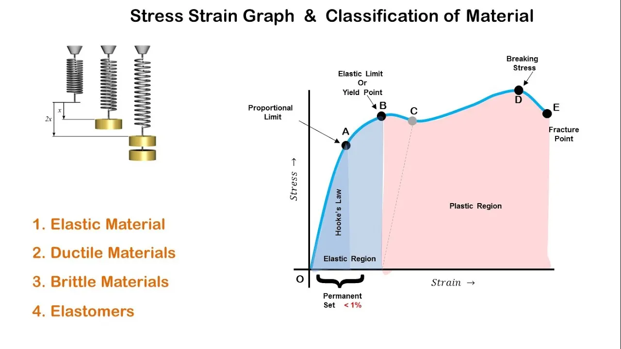
assumptions made to run for linear static analysis.

• The defomration is small
• The loading and boundary conditions are invariable in magnitude and direction during the analysis.
• The material properties are elastic.
• The relationship between the loads and the displacement follows hookes law.

Let us understand with FE solver representation.

• The FE solver will always follow a straight line form base to deformed state.
• In real life after crossing the yeild point, the material follows a non linear curve but solver follows the same strraight line.
• It can be solved analytically.

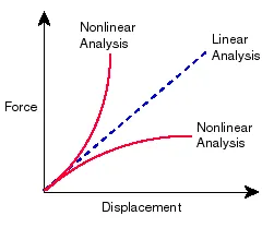
Linear analysis means the curve which is in linear upto yeild point after that the curve under plastic deformation and breaking point.but the software follow linearity through the stress strain curve it is used for static calculations.

Not always static loads standing on bar, beam, component too much deformation., but in real life if our static load crosses yeild point we dont use linear analysis.

after crossing the yeild ppoint we got a garbage value.

Non linear analysis: Mathematically speaking , a nonlinear system is one which behaviour is not equal to the sum of its parts.therefore, the behaviour of a non linear system does not satisfy the principle of superposition. in linear analysis , it is assumed that the response of the structure (deformation, internal loads, or stresses etc) is linearly propertional to the applied loads .however in real life , this responses may not be linearly proportional to the applied loads and then the structure must be analyzed using non linear assumptions.

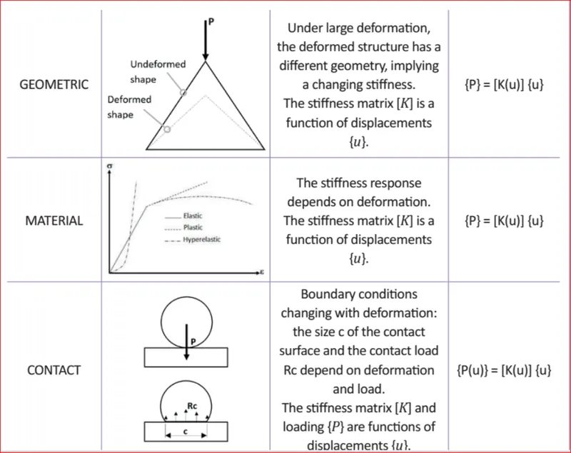
In structural analysis, the nonlinearity effect can occur due to three types of non linearity

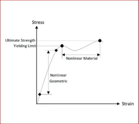
CASES:

In linear static analysis,the stiffness [k] of the analyzed structure is assumed to be constant, but in real world conditions will dependent on material , geometric and contact .

In nonlinear analysis, these changes are taken into account, and the stiffness matrix is updated using the deformed structures configurations after each incremental load applications.

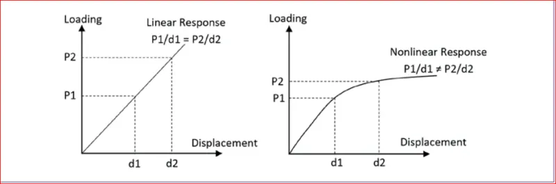
1) Geometric non linearity: if continous body undergoes large deformations, the strain-displacement relation become non linear. moreover, under large deofromations, the stiffness of the system will change with deformation, making the problem non linear.

• The sstiffness[k] is re calculated after a certain predefined displacements as an example think of a buckling case. The stiffness of a geometry changes dramatically when or after buckling has occured the new deformed geomety must now be taken into account in oder to get reasonable results.

2) Material non linearity:if the material does not follow hookes law, non linear material models must be used.

• This is related for instancenonlinear elastic, elasto plastic, visco elastic behaviour. the force (stress) vs displacement (strain) curve is non linear polynomial.

3)Boundary nonlinearity: The most frequent boundary nonlinearities are encountered in contact problems.

• In contact analysis, the stiffness [k] is also changes as a function of displacment.

3)STATIC ANALYSIS:The external effect applied to the system does not dependent on time. Something stationary the loading / force is almost constant.

ex: A cantilever beam having hook in that we have a clock.

Real world example:

Desing a bracket to mount it on a fuel tank.

• The force is static i.e, there is no variation with respect to time (dead weight).
• Equlibrium conditon `sigma`forces (Fx,Fy,Fz) and movements (Mx,My,Mz).
• The FE model must fullfill this condition at each and every node.
• The complete model summations of the external forces and moments is equal to the reaction force and moments.
• The basic finite elements equations to be solved for structure experinencing static loads can bve expressed.as
• K*U=P

4) Dynamic analysis:

Linear dynamic: Forces increase linearly with parametrs such as position and velocity.

eg: force acting on a mass on a linear spring.

Nonlinear dynamics:In non linear system where on or more forcing elements does not vary linearly with space parameters

eg: force on the same mass with non linear spring ;

k varies with displacement, frictional forces, dampping elements, resistive elements in circuits.

METHOD OF TIME INTEGRATION:

TIME DISCRETIZATION: A dynamic problem is resolved into multiple time steps for accurate calculations.

they are two methods for calculating the time step.

1) Implicit method: Acceleration is assumed to vary linearly over time step. we solve the following equations for acceleration of a single dof system.

actual acceleration

gravity - positive acceleration

decelaration-hitting, stopping etc.

example: slamming the door -door rim, outside the door comes under small deformations.

EXPLICIT METHOD: Acceleration is assumed to be aconstant over a time step. we solve the following equations for acceleration (central difference method).

Vt + dt/2 = Vt-dt/2 + at +dt.

SHAPE FUNCTION: Better the shape function more the accuracy the shape function for an element is responsible for interpolation of nodal results.

The discretization of the problem into several nodes defined by FEA analyst means that the computer will solve the problem at these particular nodes. the nodal results must also be defined in the element, which connect the nodes. for this purpose, a mathematical object called a shape function is used to represent assumed behavior for a given element. how well each assumed shape function matches the true behaviour directly affects the solution accracy.

To represents the deformation of elements under loading, we must therefore choose a mathematical function for each element. for each element, appropriate shape function is defined to represents the distrubution of displacement within the elements ,using an appropriate mathematical function. the most commonly used functions are polynomials.

Depending on the number of degree of freedom of the elements ,we derive different shape functions to express the shape of the assumed dispolacement fileds over the domain of the elements.

It is important to choose functions that gurantee the continuity of displacement for all degree of freedom at each node of the element. in other words the shap[e function must prevent openings,overlaps,and jumps.

GAUSSIAN INTEGRATION:It helps in calculating the nodal results more accurately,easily, it is used for quad, trias.

INTRODUCTION TO RADIOSS:

1) First radioss run, time steps

2) Element properties

3) material properties.

4) hypercrah

5)interface modelling

6) kinematic conditions

7) load definition

8) Methods to increase simulation speed-time step control

9)Out put requests

10) Debugging an error.

PROCEDURE FOR THIS CHALLENGE:

1.Using the crash beam file from the previous assignment, change the run time to 55 ms.

2. Change the number of animation steps during simulation to a minimum of 25 and maximum of 60.

They are menctioned above two run time and animation step.

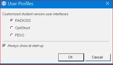
firslty opent the hypermesh and set it to radioss.

below figure represents the opening of radioss.

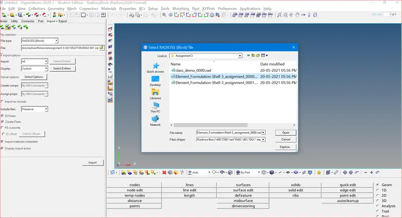
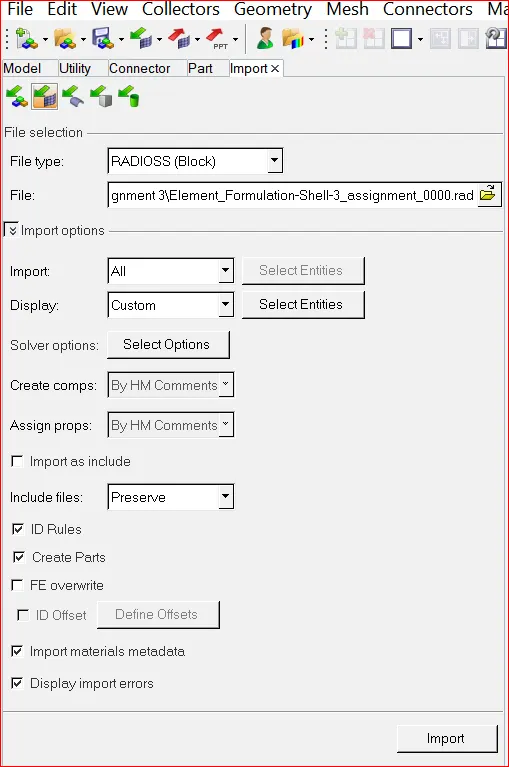
After selecting radioss then we will import a solver deck with file.

procedure for importing a solver deck.

After importing the model we have to press the f for fit.

after importion of the cad model it will be appeared like this.

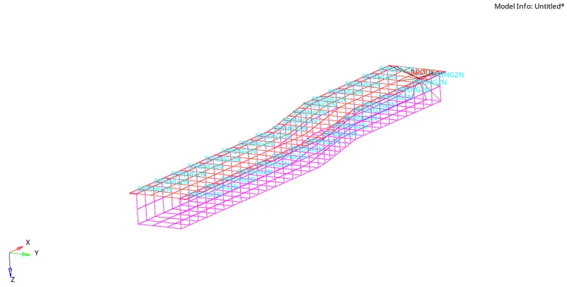
after successfully importion of a cad model we need to put it in element

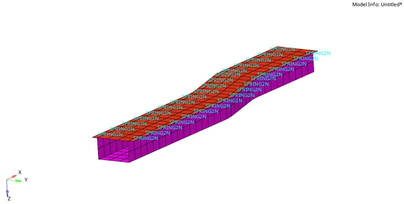
Step-2:After importing a file we need to edit the engine cards of time step as 55 and engine animation is 35.

as per the question need to change the engine run to 55 and animation steps to 25-60 in between. i took 35 is my animations step.

so my time frequency is = runtime/frames = 55/35=1.5714.

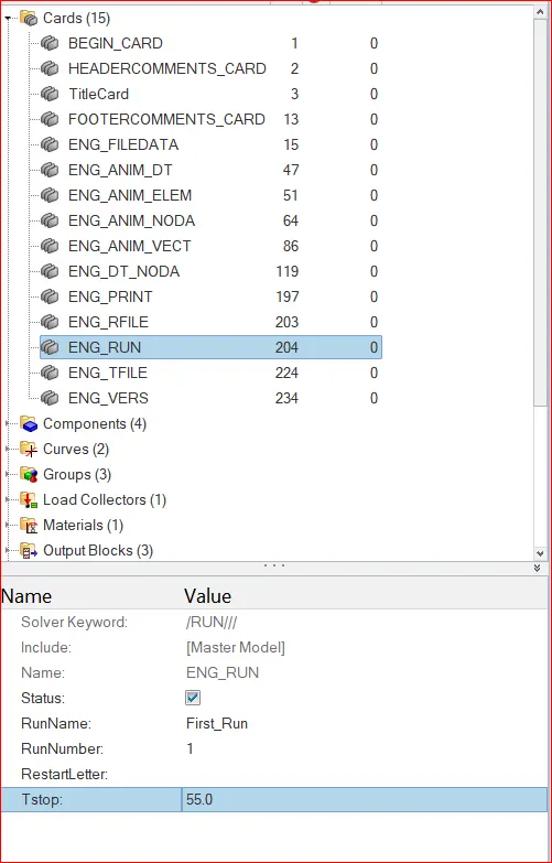
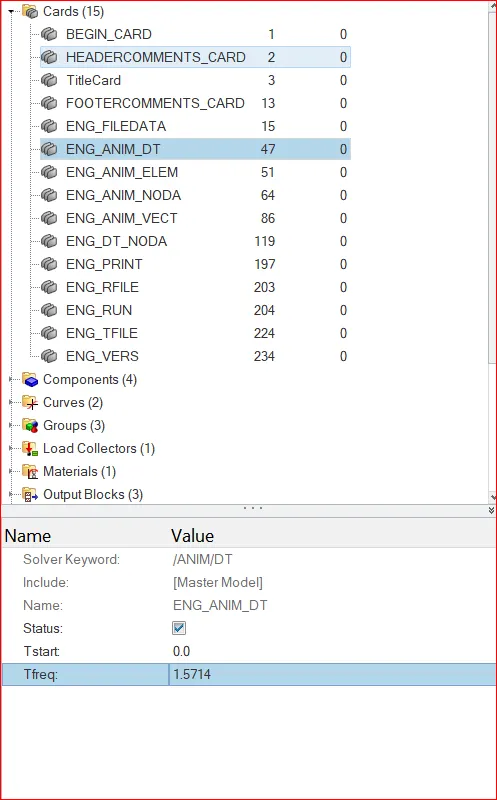
after changing the time step and engine run time. without changing the properties of the material and element cards we can run the simulation.

Step -3 3. Run the base simulation without any modification to element properties.

As per the question without modfying the element properties we run the simulation by using analysis of radioss command.below figure represents the default material properties.

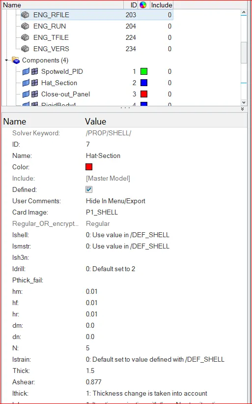
after went to the radioss , we have to save our model and in the options we can change it into nt 4 for four cores and for faster run time.

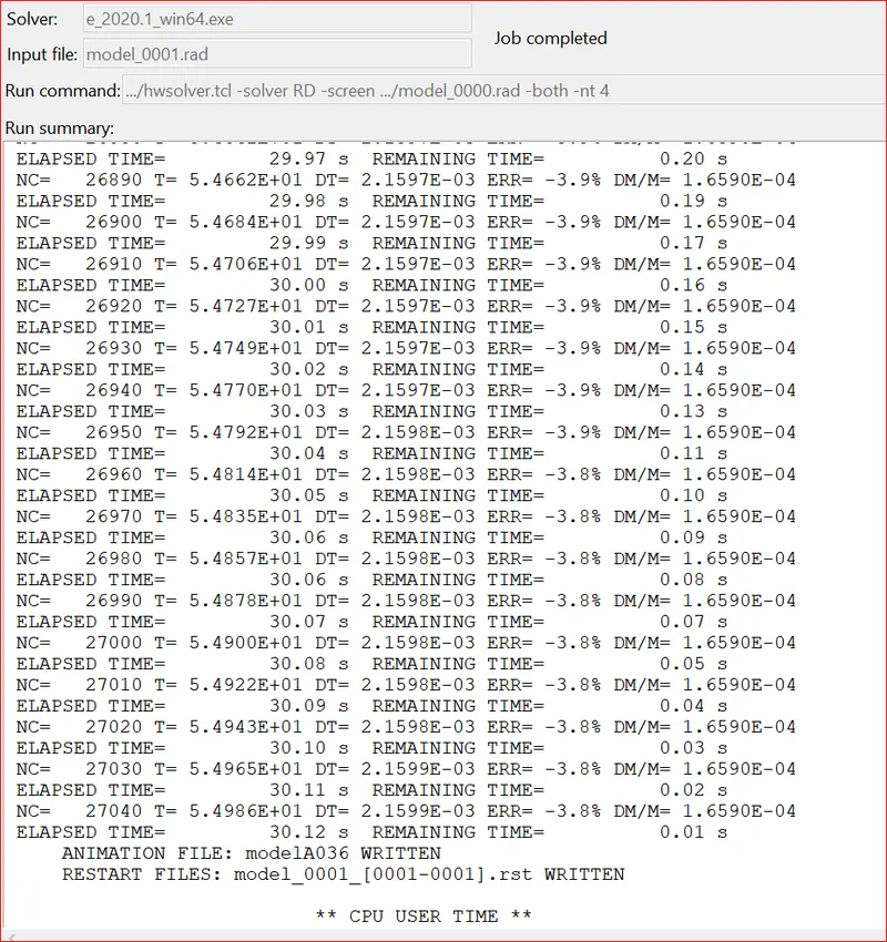
Step-4 Now we have to check the energy error and mass error.below figure represents the energy error and mass error.

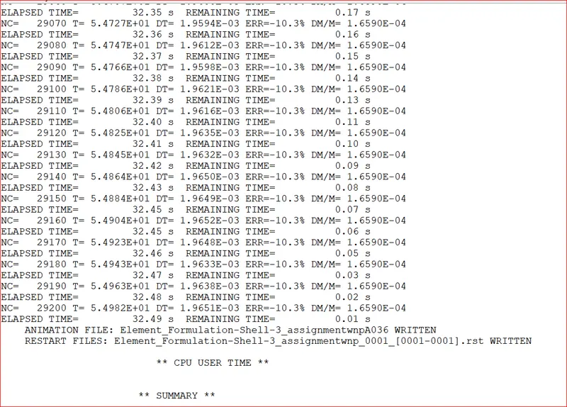
• Here i got energy error is 10% which is acceptable. for this analysis we can accept upto 15%.
• For mass energy it is in the range of 1.6590e-04 which is also in acceptable range.

we can proceed to take the displacement and hourglass energy plots.

5.If acceptable, Plot rigid wall forces, internal energy, hourglass energy, contact energy, total energy of the simulations.

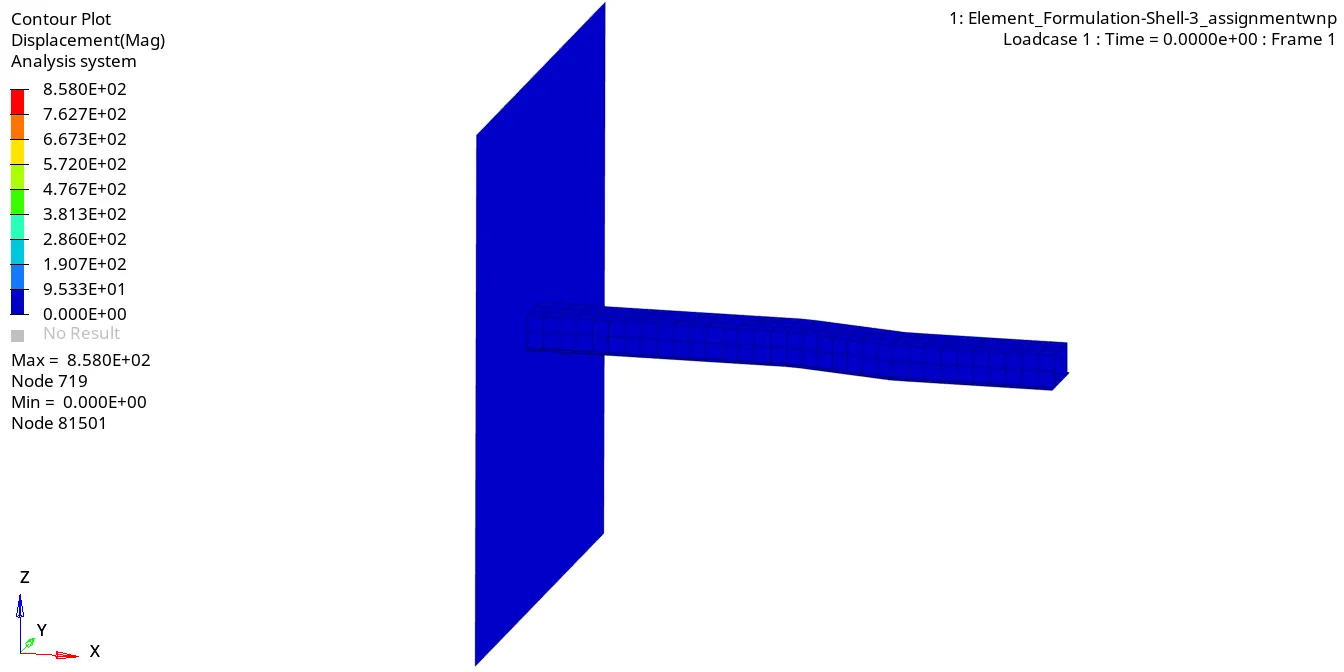
Step-5: after completing the complation using coding we can directly press the result tab it will directly open hyper view and where we can we observe the movement of the component.

Displacement contour plot with no property change.

Hour glass contour animation file wiht no property change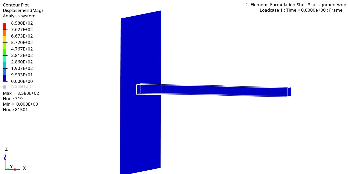

Step-6: After saving the animation file we will move on to the hypergraph 3d for plot the total energy, rigidwall forces, hourglass energy, contact energy.

for this we have to open the T01 file for plotting the graphs.

Rigid wall force without changing the properties of element and material

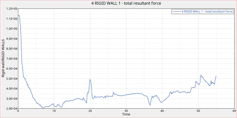
The above figure represents the graph plotted betweeen rigid wall force on y axis and time in x axis.if we observe the graph from starting to ending the rigid wall force increased and decreased a lot of disturbance , due to this we can conclude that without giving the properties it should be like this.

Step-7: After successfully pltting the graph for rigid wall force vs time.we will move on to take the graph for internal, contact, kinetic, hourglass energies.below figure represents these energies.

Internal,hourglass,kinetic,contact,total energy without changing the properties

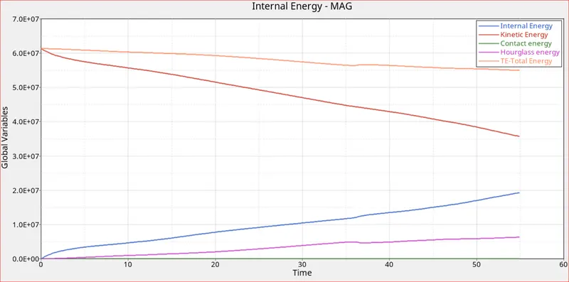
From the above graph reprenting kinetic , hourglass, total, contact, internal energies without changing the properties of material and element.

we can conclude by observing above graph there is is drastically increasing in hourglass energy called artificial energy by balancing the other energies.

CASE -2-CHANGING THE PROPERTIES OF A MATERIAL.

Recommended properties:

Parameters		Comment
Ishell =24		QEPH 4 nodes shells are best combination of cost and accuracy.
Ismstr=2		Full geometric nonlinearities (default)with possible small strain formulation activation in RADIOSS Engine.
Ish3n=2		Standard 3 noded shell (C0)with modification for large rotation(default)
N=5		Number of integration points set to 5 for accuracy bending.
Ithick=1		Thickness change is taken into account for accuracy.
Iplas=1		Iterative plasticity for good accuracy.

Step-8: We have to assign the above given material properties to the component.below figure represents the assigned material property.

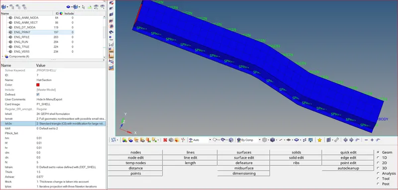
From step -1 to step -4 same procedure we have to follow to this also after assigning the engine run time -55, and frames to -35 and frequency of time to 1.57. we need to assign the properties of the element. after successfully assigning the element properties. we again go to radioss and analysis follow the same procedure like previous.

for next we will click the results it will directly open the hyperview and we can observe the displacement contour animation file.

Displacement animation file with properties

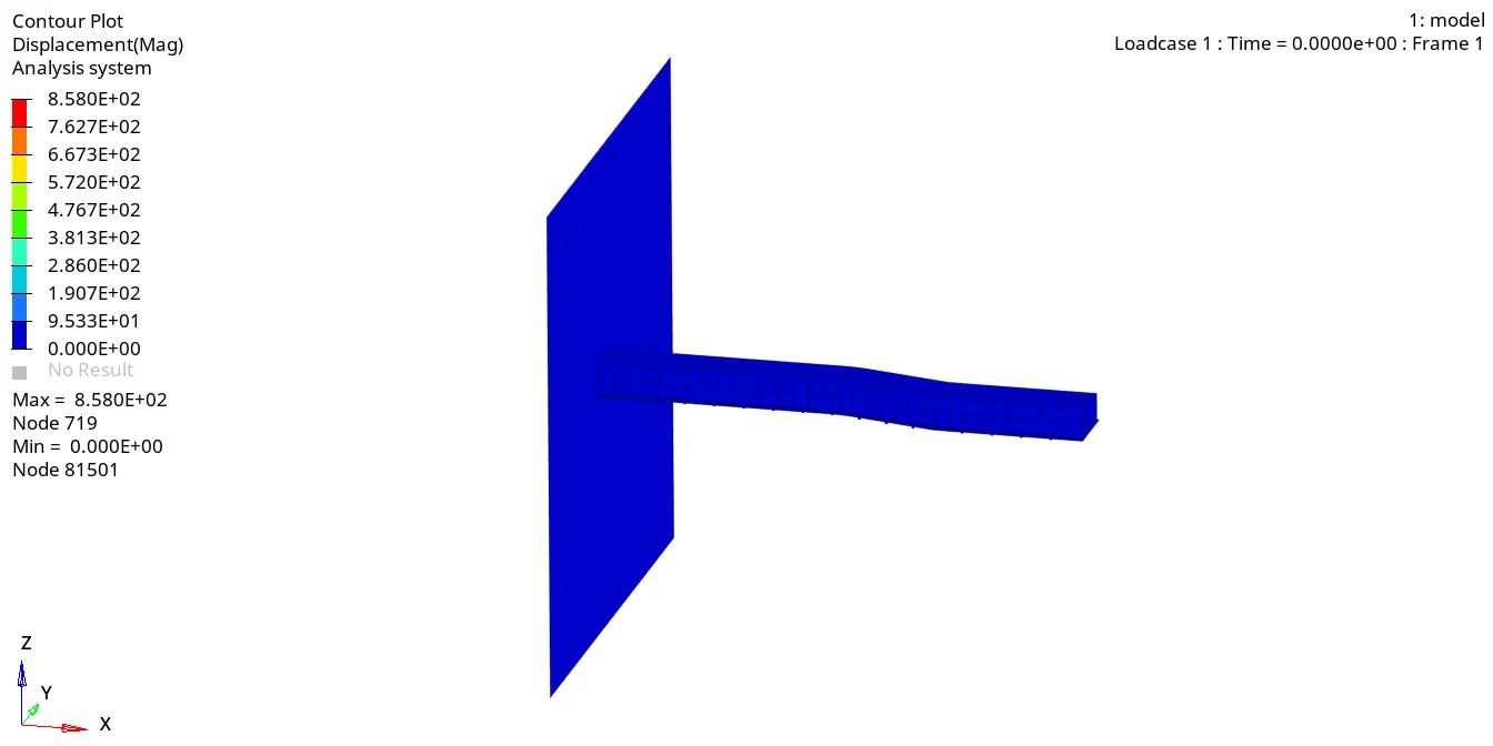
below figure represents the hourglass, kinetic, total enegy graphs.

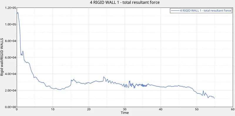
Rigid wall force with properties

Internal, kinetic, contact,hourglass,total energies with properites

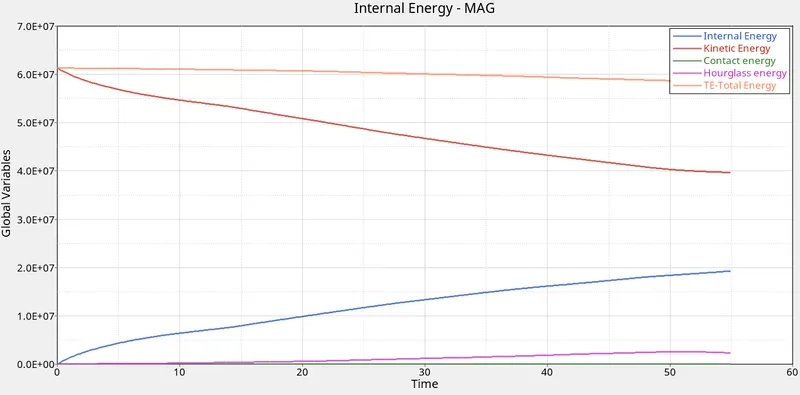
RESULT:9. Comment whether there is any change in the results and why there is any change in the result.

Without properties With properties

so we can conclude that compared to without properties graph , with properites of internal energy graph given more accurate and optimum results.

so when ever we assigned the i shell, and i thick and ismstr properties the integration points calculate the displacements and other energies with accurately.

so we conclude that hour glass enenrgy is increased in left side due to lack of integration points and without assigning of element properties.so we conclude that the hourglass energy is less in right graph.

final judgement: artificial energy(hour glass energy ) it does the energies balance. and lesser hour glass energy means results will be stable and more accurate and optimum.

LEARNING OUTCOMES:

• What are types of analysis
• what is time integration
• what is shape function
• introduction to radioss
• how to import a .rad file
• how to assign the run time and frequency time in engine run and engine dt cards.
• how to save radioss file
• how to compute the radioss analysis
• checking with energy error and mass error compared with ideal error.
• how to go to the hyperview and save the animation file.
• how to save the displacement file.
• how to go to hypergraph.
• how to plot the required energies,rigid wall force graph.
• how to compare the two graphs with and without properties
• what is hour glass energy.